
Rollercoasters and railways were originally created without using curvature calculations. People on them would experience undesirable jerk (a sharp change in curvature results in jerk or centripetal forces). You may still experience this on old railways. The image below depicts a centrifugal railway that was constructed in 1846. Nowadays, rollercoaster and railway designers use a type of curve called a clothoid or Euler spiral to make the change in curvature less abrupt, for example when riding a loop-the-loop. I will later mention a couple of applications of Euler spirals. So curvature is clearly an important concept. Let’s get to grips with how it works, and where we should consider it.

A sketch of a centrifugal railway in Manchester, 1904.
Suppose you’re in a car that travels along a meandering, curved road. The fact that the road is curved affects your car and you feel the force of curvature, which can be defined as the degree to which the road deviates from a straight line. Since following a curved line means changing direction, you undergo a change in velocity. The formula below combines velocity ($\mathrm{d}y/\mathrm{d}x$) and acceleration ($\mathrm{d}^2y/\mathrm{d}x^2$) in a way that expresses this ‘degree of curvature’, which we typically denote with the Greek letter $\kappa$—‘kappa’. We will derive this formula later.
$$\kappa = \frac{\frac{\mathrm{d}^2y}{\mathrm{d}x^2}}{\left(1 + \frac{\mathrm{d}y}{\mathrm{d}x}^2 \right)^{3/2}}$$

The osculating circle to the curve $C$ and the point $P$, with radius $r$.
Curvature can be expressed in terms of the radius of an osculating circle, which is the circle that is tangent to a curved line. The image on the right shows the osculating circle at the point $P$ on the curve $C$. The radius of the circle is $r$. Different degrees of curvature result in circles with varying radii. This is a good way to describe how much you’re turning as you travel along the curve. Thinking back to our example of a car driving along the road, a small turning (osculating) circle means that the car is making a sharp turn. Curvature is the reciprocal of the radius of this circle. Since curvature is a measure of how much something turns, a sharper turn should mean greater curvature. But a sharper turn produces a smaller radius, so we take the value of curvature to be the reciprocal. By contrast, a relatively straight road would trace out a circle with a larger radius, corresponding to a small curvature.
Proof of the curvature formula
Before we look at some more applications of curvature, let’s derive the algebraic expression for $\kappa$. Well, actually we will derive the expression for the radius of curvature $\rho$ (‘rho’) and then we just have $\kappa = 1/\rho$ by the argument above. We want to see how $\rho$ changes as we move along the curve, which has arc-length $s$ and angle $\theta$ measured from the horizontal.
By Pythagoras theorem, the change in arc length is $\mathrm{d}s^2 = \mathrm{d}x^2 + \mathrm{d}y^2$ — that is, this is the expression for how the length of the curve $s$ changes as we adjust $x$ and $y$ by some small amounts $\mathrm{d}x$ and $\mathrm{d}y$.
By trigonometry, we can express $x$ and $y$ in terms of $\rho$ and $\theta$: $x = \rho \cos{\theta}$ and $y = \rho \sin{\theta}$. The product rule applied to these two expressions gives us
$$ \frac{\mathrm{d}x}{\mathrm{d}\theta} = \cos{\theta} \frac{\mathrm{d} \rho}{\mathrm{d}\theta} – \rho \sin{\theta}, \\ \frac{\mathrm{d}y}{\mathrm{d}\theta} = \sin{\theta} \frac{\mathrm{d} \rho}{\mathrm{d}\theta} + \rho \cos{\theta}.$$
Multiplying through by $\mathrm{d}\theta$ and combining these in the arc-length formula we find
$$\mathrm{d}s^2 =\mathrm{d}\rho^2 + \rho^2 \mathrm{d} \theta^2,$$
where for infinitesimal changes along the curve $\mathrm{d}\rho$ is very small so that $\mathrm{d}s = \rho \mathrm{d}\theta$. So we just need to find $\rho = \mathrm{d}s/\mathrm{d}\theta$. But we already know $\mathrm{d}s$! It remains to find $\mathrm{d}\theta$, that is how the angle changes as we move along the curve.
Again, trigonometry helps us out. We know that $\tan{\theta} = \mathrm{d}y/\mathrm{d}x$. Differentiating both sides with respect to $x$, and using a trig identity (a nice exercise!) we get:
$$(1 + \frac{\mathrm{d}y}{\mathrm{d}x}^2) \frac{\mathrm{d}\theta}{\mathrm{d}x} = \frac{\mathrm{d}^2y}{\mathrm{d}x^2}.$$
Combining the expressions for $\mathrm{d}\theta$ and $\mathrm{d}s$ we get:
$$\rho = \frac{\mathrm{d}s}{\mathrm{d}\theta} = \frac{\left(1 + \frac{\mathrm{d}y}{\mathrm{d}x}^2 \right)^{3/2}}{ \frac{\mathrm{d}^2y}{\mathrm{d}x^2} },$$
which is just the inverse of the expression for $\kappa$ that we started with.
Phew! Now let’s think about why curvature is important in the real world, and some of the places where designers have to take it into account.
The Mercator projection
Throughout the 16th century, cartographers began creating maps of the world which included distortions of land. In 1569 the Dutch geographer Gerardus Mercator came up with a (not-so-perfect but still pretty good) solution to the problem of mapping the earth, a three-dimensional planet, onto a two-dimensional map. It is known as the Mercator projection.
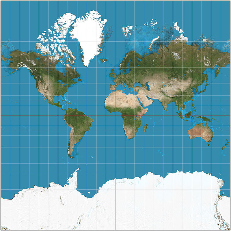
The Mercator projection distorts countries that are close to the poles. Image: Strebe, CC BY-SA 3.0.
A map is a two-dimensional object, so it is flat with zero curvature. But the mean curvature of the globe isn’t zero—you can’t ‘lie it flat’ without distortions. This means it is impossible to create a flat map of the round Earth without distorting it in some way. There is an inevitable sacrifice of either relative area of locations, depending on proximity to the poles, or relative location of areas being distorted, which results in countries being jumbled.
The Mercator projection can be conceptualised as projecting the globe onto a cylinder, then unrolling it to create a flat surface. Suppose you had a globe with a lightbulb in the middle of it. The lightbulb emanates light and maps countries through shadows and areas of light. We can then unroll the cylinder to produce a two-dimensional map. Distortion of area occurs as you get closer to the poles because the size of the ‘shadow’ produced by the land as it is projected onto the cylinder is larger than at the equator. This is particularly true for countries such as Greenland which appear to be larger than they actually are. While this a disadvantage of the Mercator projection, it is advantageous to use for navigation as it preserves direction and keeps the shape of countries. The website thetruesize.com allows you to play around with the Mercator projection, moving countries around to get a sense of how distorted they are.
The Euler spiral
On the other hand, if we sacrifice location and instead attempt to create a map which could propose accurate relative sizes of land, we could cut up the globe into an Euler spiral. This is where the curvature changes linearly with length. To make an Euler spiral from a globe, start at the North pole and cut around the globe in a spiral, moving downwards as you go. You’ll end up with a spiral shape, which you can flatten out. The distortion of the area of locations decreases by the inverse square of the number of spirals. That is, the amount the globe has to deform to be represented on a two-dimensional plane tends to zero as we make infinitely many spirals. Numberphile have a video explaining this, here.
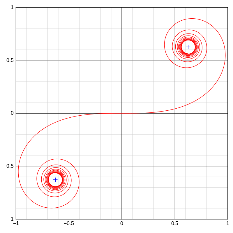
A double-ended Euler spiral. As the number of loops grows, the curve tends towards the points marked with a cross. Image: AdiJapan, CC BY-SA 3.0.
Euler spirals are used by engineers in road design. They allow for smoother transition curves and reduce the deceleration of cars as they change direction onto another road. An object travelling in a circle experiences centripetal acceleration (towards the centre of the osculating circle), and Euler spirals are useful because they allow a vehicle to change direction by increasing this centripetal acceleration linearly (gently) with the curve length. You can imagine if one was to turn directly at a tangent it would cause strain to the vehicle and the passenger would feel an uncomfortable change in centripetal acceleration (jerk). This is the same principle at play in the roller-coaster I mentioned earlier.

A roundabout constructed using clothoids or Euler spirals. Image: Anders Sandberg, CC BY-NC 2.0.
More curves
Other applications of curvature include in car design and graphic design. French engineer Pierre Bézier created a type of parametric curve while designing cars for Renault in the 1960’s. Bézier curves are created by using ‘control points’. The number of control points is equal to one more than the curve order (so four points for a cubic curve). A quadratic bezier curve will be described by 3 control points: $P_0$, $P_1$ and $P_2$. Starting at $P_0$, the curve moves towards $P_2$, passing close to $P_1$. The Bézier curve is defined in such a way that the curve gets close to the control points while maintaining a smooth change in curvature so that it still looks natural. Specifically, the curve is constructed by moving along a line (the green line below) that connects the straight lines between successive control points (the grey lines). If the curve is described by a parameter $t$, then the relative position along each of the construction lines is the same (watch how all the dots move as the $t$ increases in the animation below — at $t = 0.5$ the green dots are halfway between the control points, and the black dot which traces the curve is halfway along the green line). Bézier curves are also used in graphic design to make complex shapes, draw smoother lines and create the feeling of realistic motion.

The construction of a quadratic Bézier curve.
In conclusion, the use of calculus has made the concept of curvature mathematically explicit, and this has given us smooth rollercoasters, allowed us to understand maps with greater accuracy and much more besides.
More from Chalkdust

How to be more Pythagoras
Max Hughes investigates how channelling your inner Pythagorean may help you to become the next big lifestyle influencer
Danny Chung Does Not Do Maths
We review the first of this year's nominees for the Book of the Year
Can computers prove theorems?
And will we soon all be out of a job? Kevin Buzzard worries us all.
Variations on Fermat: an agony in four fits
Fermat's Last Theorem with complex powers, wrapped in a story every mathematician can relate to
Roots: the legacy of Fibonacci
More than spirals and rabbits, Fibonacci gave us something much more fundamental.
£100 Prize Crossnumber, Issue 01
Our original £100 prize crossnumber. Download and enjoy!