
A good puzzle leads you to explore unexpected places and discover hidden gems of mathematics – Me, just now

Image: Wikimedia commons user Dougism. CC BY-SA 4.0.
By that reasoning, Catriona Shearer’s puzzles rate extremely highly. Many of them have sent me on an intriguing journey through mathematics, right from the very first that I encountered. The resulting magical mathematical expedition is what I hope to show you in this article.
The puzzle itself is given below. For such a lovely puzzle (as we’ll see), it didn’t get much traction. Indeed, the next day Catriona posted an update with some of her ideas about solving the problem. That second tweet was sufficient to pique my curiosity. After a couple of back-and-forth tweets, I learnt that the problem had been inspired by the bell ringing pattern. With a little time to spare (these were posted in the school holidays!), I set to and investigated. I was pleasantly surprised to find myself embarking on an adventure that started with a morning of bell ringing, continued with a merry afternoon of braiding, and ended the day with a mad dash in a taxi.
Dotty puzzle by Catriona Shearer
 From one row to the next, each point swaps with the neighbour it didn’t swap with last time. What percentage of the grid is enclosed by the red and orange lines? By red and yellow? By other pairs of colours?
Let’s ring in the changes
Those around me have gotten used to me declaring “but that’s mathematics” to the point that they are quick to reply yes, but you say that everything is mathematics”. Which is fair enough: I do have a tendency to think that. But with bell ringing, I’m not on my own in this claim.
In bell ringing, the bells are rung in changes or rows. Each change consists of every bell being rung once in some order. From one change to the next, bells can swap position with a neighbouring bell. We can draw this in the fashion of Catriona’s pictures wherein each row is a change and each bell is a dot in that row. The first diagram below shows three such changes. A picture that doesn’t paint a thousand words is missing something. In this case, it’s very tempting to `join the dots’ and that’s a helpful thing to do as it shows the progression of each bell. Of course, colour is always a welcome addition as in Catriona’s original picture. Indeed, with the colours we don’t need the labels. The second diagram shows the end result.


All tangled up
Images such as the above are reminiscent of braid diagrams. A braid in mathematics is very like a braid in “real life”: it consists of strands travelling in a given direction which can cross over or under each other. The picture below gives a simple example.
If you haven’t encountered braids before, here is a quick precis. They form a part of both topology and algebra. In topology, they are closely related to knots and links. Knots in mathematics model knots in the `real world’, the main difference being that we join the ends to stop them undoing themselves. Links generalise knots in that they can have multiple strands. A braid can be made into a knot or a link by joining the strands from the bottom back up to the top and the crossings of the braid then create the knottedness of the resulting knot. Braids also find a place in algebra. The set of braids on a fixed number of strands forms a group, with the group operation being concatenation: placing one braid after another. These groups have a lot of structure which provides a rich source of study.
Knots, links, and braids have many applications both in wider mathematics and further. One such application is in the study of DNA: the helix structure of DNA makes it naturally braided. When DNA is replicated as part of cell division, it remains tangled so has to be untangled for it to properly separate and be able to pass into the two new cells. There is a particular enzyme that does this, so a mathematical concept—unlinking—is realised by a particular biological process.
The bell ringing diagrams are not quite braid diagrams, however. The difference is that in bell ringing there is no information as to which strand crosses over which. Despite the temptation of modelling the swaps by actually intertwining the bell ropes, this would quickly lead to them being unringable. There is no movement in the swaps in bell ringing and so there is no obvious choice of which strand should go over which.

There are a variety of ways that the choices could be made, and readers might find it an interesting diversion to come up with rules to follow and to see what different braids result from the same bell ringing diagram. In what follows we will be most interested in something called the linking number of two strands. This is a concept on loan from the theory of links which measures how intertwined two strands are. It is straightforward to calculate with braids: pick two strands and follow them down the braid diagram. Each time they cross count 1 if the right crosses over the left and -1 if the left crosses over the right. At the end, halve the number. This is the linking number of the two strands. Some examples are given above, showing why it measures their entanglement.

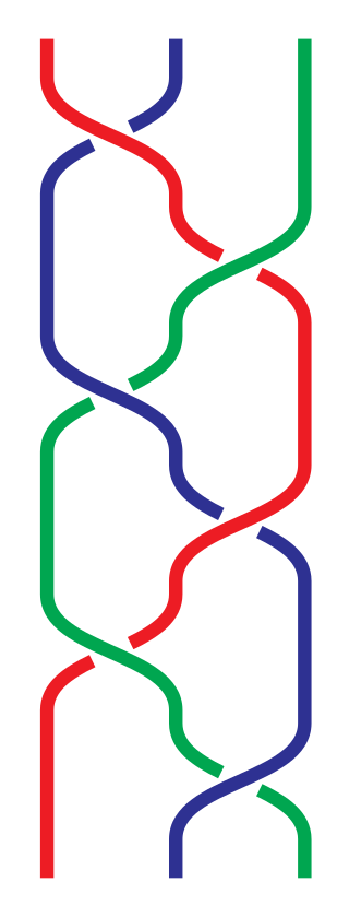
A very simple rule to use when converting a bell-ringing diagram to a braid diagram is to make every crossing “right over left”. This would ensure that the linking number between any two strands is as large as it can be. A possible line of enquiry would be to see how the linking number is affected by other choices of rule. With this rule, Catriona’s original puzzle translates to the braid shown above.
Enter the taxi
The original problem asked about the area swept out between two strands as the braid progresses. (It is worth pointing out that this doesn’t depend on the choices of crossings in the braid.) There was also the “must swap if possible” rule but we can equally well work with patterns that don’t have that property. We shall, however, assume that our braids are drawn in the more angular fashion of the original braid, which matches the style of the original problem.
To talk about area, we need to decide on some units. We’ll assign length 1 to everything atomic: the horizontal distance between adjacent strands and the vertical distance between the lines corresponding to the bells being played. Now let’s look at two strands, say the red and orange strands. The first part of their journey looks like a trapezium, as in the following picture.

Our choice of units make the area easy to calculate: it is simply the average of the two horizontal sides. More generally, for any two strands then the area of one segment where they don’t cross is the average of their horizontal distances at the start and end of that segment. The crossings behave differently, see the picture below. In this case, the area given by the above rule is 1 but the actual area is 1/2. As is common in mathematics, we’ll make that 1/2 look more complicated to make life simpler later on. We’ll write it as 1 – 1/2 where we think of the 1 as being the area given by the trapezium rule and the -1/2 a correction for the crossing. 
To see what this looks like, let’s establish some convenient notation. We’ll convert each thread in the braid into a list of numbers. These will record the position of each strand as it passes down the braid. Equivalently, the list is of the position of the bell in each change. The lists for the braid above are (from left to right):
\begin{align*}
1 2 3 4 5 5 4 3 2 1 1 \\
2 1 1 2 3 4 5 5 4 3 2 \\
3 4 5 5 4 3 2 1 1 2 3 \\
4 3 2 1 1 2 3 4 5 5 4 \\
5 5 4 3 2 1 1 2 3 4 5
\end{align*}
Notice that the last change is the same as the first. Let’s look at the calculation of the area between the first two strands. Separating it by change, it is:
\begin{align*}
{|2 – 1| + |1 – 2|}/2 &- 1/2 \\
+ {|1 – 2| + |1 – 3|}/2 & \\
+ {|1 – 3| + |2 – 4|}/2 & \\
+ {|2 – 4| + |3 – 5|}/2 & \\
+ {|3 – 5| + |4 – 5|}/2 & \\
+ {|4 – 5| + |5 – 4|}/2 &- 1/2 \\
+ {|5 – 4| + |5 – 3|}/2 & \\
+ {|5 – 3| + |4 – 2|}/2 & \\
+ {|4 – 2| + |3 – 1|}/2 & \\
+ {|3 – 1| + |2 – 1|}/2
\end{align*}
What is important to note in this is that the second term in each fraction is the first term of the next. This even works with the last and first terms. Writing $u^a$ and $v^a$ for the terms in each list, we therefore have that this part simplifies to
$$
\sum^{10}_{a=1} |u^a – v^a|$$
Note that we’ve used the fact that the first and last terms in our lists are the same here. The other part is the linking number of these two strands, at least the way that we’ve drawn the crossings. As the area doesn’t depend on the choices of crossings then this might not always be the linking number of the given choices. What we can say is that it is the maximum linking number. Let’s write this maximum linking number of the strands which start at positions $i$ and $j$ as $Χ_{i,j}$.

Now let us return to the first part of the expression for the area, given in the equation above. This is where the taxis arrive. The taxicab metric—more formally known as the $\ell^1$ metric—is a way of measuring distance between points. In 2D, the image is of points laid out on a grid, much like a city such as New York, as in the next diagram. You can move along the lines on the grid but you can’t move across them. The distance between two points is therefore not the standard Euclidean distance but a different formula. More prosaically, it is not “as the crow flies” but rather “as the taxi drives”. The distance between the two points in the diagram to the right is 2 + 1 + 2 + 2 = 7. No matter what choice of route, no shorter distance can be found. This gives rise to the formula for the taxicab distance between two points $a=(x_a,y_a)$ and $b=(x_b ,y_b)$ as:
$$|a – b|_1 = |x_a – x_b| + |y_a = y_b|$$
There’s nothing special about 2D here. The analogous formula holds with arbitrary length vectors. Thinking of a vector as just a list of numbers (i.e. without trying to assign any physical meaning to the directions), our listing for each strand of our braid gives a vector.
The expression in the above equation shows that we should drop the repeated ending position and so the vectors from the braid in Catriona’s original puzzle are of length 10. Our vectors from that braid are therefore:
\begin{align*}
v_1 &= (1,2,3,4,5,5,4,3,2,1) \\
v_2 &= (2,1,1,2,3,4,5,5,4,3) \\
v_3 &= (3,4,5,5,4,3,2,1,1,2) \\
v_4 &= (4,3,2,1,1,2,3,4,5,5) \\
v_5 &= (5,5,4,3,2,1,1,2,3,4)
\end{align*}
The area formula then simplifies to: $A(v_i,v_j) = |v_i – v_j|_1 – Χ_{i,j}$. Calculating this for the above vectors (exploiting a bit of symmetry to avoid too many calculations), we get:
\begin{align*}
A(v_1,v_2) &= A(v_2,v_4) = A(v_4,v_5) = A(v_5,v_3) = A(v_3, v_1) = 15 \\
A(v_1,v_4) &= A(v_4,v_3) = A(v_3,v_2) = A(v_2,v_5) = A(v_5,v_1) = 23
\end{align*}
In conclusion, the area between two strands is given by taking the taxicab metric applied to the corresponding vectors and then subtracting their maximum linking number.
And finally
As I said at the outset, the mark of a good problem is that it gives you the opportunity to travel in mathematics.
This particular problem took me on a meandering wander through some parts of mathematics that I know well, but that I hadn’t realised were so closely connected. It is easy to forget how intricately connected mathematics is, and I find expeditions such as this one help to remind me of this.
While I knew of the connection between bell ringing and braids, I certainly wasn’t expecting to see the taxicab metric making an appearance.
Moreover, its role here is to calculate an area whereas its natural home is as a way to measure length, so it also served to remind me that area and length are more closely tied together than I often allow. This journey has also led me to places that I’d like to revisit when I have a bit more time. For example, the relationship between bell ringing and braids is not quite as I’d thought: I hadn’t realised the significance of the crossings. So there’s plenty to explore further with trying out different crossing rules to see what braids appear. Plus it gives me an excuse to draw some more braid diagrams, which is always a bonus.
This article is inspired by a puzzle from Catriona Shearer. The central council of church bell ringers is always looking for mathematically-minded recruits! Find them at cccbr.org.uk.
More from Chalkdust

Universal poetry
Andrew Stacey explores the mathematics within poetry.
What can you do with this space?
Nobody could draw a space filling curve by hand, but that doesn’t stop Andrew Stacey
When Truchet met Chladni
Stephen Muirhead meets neither, as he explores waves, tiles and percolation theory
Playing billiards with cue-bics
Yuliya Nesterova misses all the pockets, but does manage to solve some cubics
Hiding in plain sight
Axel Kerbec gets locked out while exchanging keys
In conversation with Matt Parker
Interviewing Matt was a mistake