
Icy patches sit in wait and bare trees shiver in anticipation but spring is still dawdling, likely enjoying a final cuppa before going back to work. What are we to do while days are dreary and the wind rummages through empty branches? Why, stay inside and play with geometry software, of course! Yet winter was long and snowy, and after one too many hours indoors the treasure trove of maths is perhaps running low.
 What to do once ancient theorems are re-proved and the excitement of a parametric plot has wilted? Well, there is still a nugget of algebra that could flourish into hours of exploratory fun. So grab your Geometer’s Sketchpads, your Geogebra, or simply some transparencies and coloured markers, and let’s play billiards with polynomials.
In the vast sea of beautiful mathematics it is quite easy to drown, finding more and more interesting papers on a subject, eventually getting lost in the plethora” of nifty theorems and charming proofs. It’s best to restrict ourselves early on in the game if we are to make an afternoon of it. Let’s say for today that we consider only the polynomials of degree 3. Armed with our restriction—cubics only!—let us dive into the deep end of adventure.
Build a billiards table
To play a good long game of billiards, you must first build a pool table (as Carl Sagan might have it). Look at your cubic polynomial, for now remaining mysteriously general: $a_3 x^3+a_2 x^2+a_1 x+a_0$. First, from the origin in the positive $x$-direction, draw a line segment $a_3$ units long. At the end of it, turn 90° anticlockwise and draw a line segment of length $a_2$. Turn 90° anticlockwise again to plot $a_1$, and do the same for $a_0$. Call the final point you arrive at $\Omega$, where you build a corner pocket. If ever a coefficient is negative, you ‘backtrack’, plotting out a segment backwards but still remembering the direction in which you face for the next turn. Now for the playing part: the segments constructed, and the lines extending them, have become walls. Our objective is to launch a ball from the origin and hit three walls, sinking it into $\Omega$, much like in three-cushion billiards. In the words of our indices, “3, 2, 1, sc0re”!
But on this special table, the physics is peculiar: our ball makes a 90°-turn each time it bounces off a wall.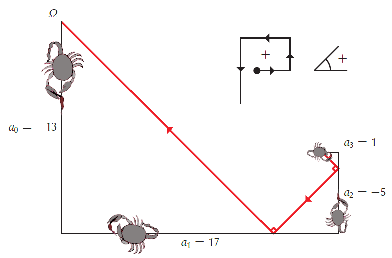
Here is a path on $x^3-5x^2+17x-13$. We try different launch angles $\alpha_3$ from the origin (3 is for cubics), bouncing against walls (hitting the corners if necessary), until we find the winning path to $\Omega$. Once a path is found, $-\tan\alpha_3$ is the real root of the polynomial! The path in the picture corresponds to the root $-\tan\alpha_3= – \tan(-\frac{\pi}{2})=1$. A visual way to factor polynomials through a geometric game.
You can handle the truth
Perhaps it is far more rewarding to know why this method works than it is to practise it. If you want the magic and mystery to remain, pause now until you’re ready. Otherwise, let’s dive deep into geometry and fish out some nuggets of truth.
With the choice for each coefficient of whether to go forwards ($+$), stay and turn (coefficient of $0$) or to backtrack ($-$) along each segment, we need casework to do the proof properly. But with long cold nights in our near future, we will talk business here and leave the details to settle into place in due time with some well-chosen parameters.
Let’s consider first the ideal case: all coefficients positive, $a_3 x^3 + a_2 x^2 + a_1 x + a_0$, our billiard ball makes two right angles to land perfectly at $\Omega$, the endpoint of $a_0$. In our 90°-bounce universe, the billiard ball path forms a series of 3 similar right-angled triangles. In each triangle, call $s_k$ the side opposite angle $\alpha_3$, starting with $s_3$ for the triangle at the origin. Let’s trace out the trigonometry.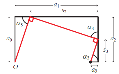
We start with $s_3 = a_3 \tan\alpha_3$. In the next triangle:
$$s_2 = (\tan\alpha_3)(a_2 – a_3 \tan\alpha_3)=a_2 \tan\alpha_3-a_3 \tan^{2} \alpha_3,$$
and $$s_1 = a_0 = (\tan\alpha_3)(a_1 – s_2)=a_1 \tan\alpha_3 – a_2\tan^{2}\alpha_3+a_3 \tan^{3} \alpha_3.$$
Replacing $x=-\tan\alpha_3$, we get exactly our polynomial, $a_0 + a_1 x + a_2 x^2+ a_3 x^3=0$, so $x=-\tan\alpha_3$ is indeed a root of the original polynomial. Simple enough.
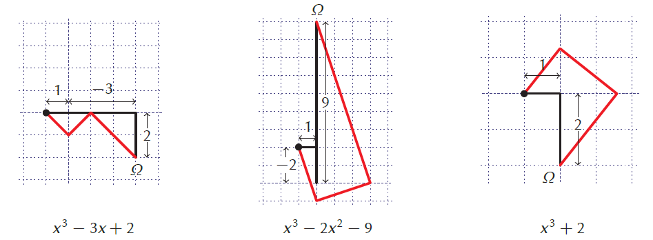
Ever catch a side length of zero? A length, you will agree, unacceptable for a stable pool table (or a pool). And yet the maths works out! If an $a_k=0$, we generalise: draw a line where segment $a_k$ would have been: a ball hitting a line-wall outside the segment $a_k$ will go right through the wall, still making a 90° angle with the path coming in. Not much of a table in this case and not much is left of billiards but the procedure still
delivers a visual way to find real roots. Three examples with zero coefficients are showcased below.
|
\begin{align*} s_3 &= a_3 \tan \alpha \\ s_2 &= s_3 \tan \alpha \\ &= a_3 \tan^2 \alpha \\ a_0 &= (a_3 \tan^2 \alpha + a_1) \tan \alpha \\ &= a_3 \tan^3 \alpha + a_1 \tan \alpha \end{align*} |
\begin{align*} s_3 &= a_3 \tan \alpha \\ s_2 &= (s_3 – a_2) \tan \alpha \\ a_0 &= s_2 \tan \alpha \\ &= a_3 \tan^3 \alpha – a_2 \tan^2 \alpha \end{align*} |
The proof for a triple-root cubic is too short to mention, though a beautiful picture would do it credit: $$a_0 = a_3 \tan^3 \alpha$$ |
How the tables have turned
Good news for the completionists in the audience: should you chance upon a cubic with three real roots, you can extend the process, building the walls of a new billiard table on the path of the ball’s old trajectory, continuing onwards: the ball’s path you have drawn becomes the walls for a new polynomial.
In the diagram above, I have done just that with $(x+3)(x+1)(x+2)$, better known as $x^3+6x^2+11x+6$. The original rectangle of a pool table can be played on via the red path. Its angle $\alpha_3$ (measured in the usual manner: anticlockwise about the origin from $a_3$) respects $\tan\alpha_3=3$, one of our roots. Build a second billiards table! For the three similar right-angled triangles with hypotenuses on the red path, we find the relationship of hypotenuses to be $AF:FG:G\ \Omega=1:3:2$. The path $AF, FG, \Omega G$ itself represents a polynomial ($x^2+3x+2$)! Well, we couldn’t quite tell that it wouldn’t have been $x^{\hspace{1pt}3}+3x^{\hspace{1pt}2}+2x$, or $x^{300}+3x^{299}+2x^{298}$, or, for that matter, $9x^{\hspace{1pt}2}+27x+18$. In fact, it is $\sqrt{10}x^{\hspace{1pt}2}+3\sqrt{10}x+2\sqrt{10}$, where $\sqrt{10}$ is $\sqrt{1+\tan^{2}\alpha_3}$, or $a_3/\cos\alpha_3$. You can find this from the diagram, or directly from the polynomial with a bit of work.
 Now, we jolly good shots have found an orange path to sink the ball: notice that $-\tan\alpha_{2}=-FH/AF=-1$: another one of our roots! Triangles $AFG$ and $FGH$ are once again similar, with the latter twice the size of the former, so $AH/H\mathit{\Omega}=\frac{1}{2}$: the yellow path describes the path of $x+2$ (up to multiplication by $cx^{\hspace{1pt}n}$, $c \in \mathbb{R}$, $n \in \mathbb{Z}$). We end by firing off a shot down the $x$-axis from A, to E, to victory, with $-\tan\alpha_{1}=-2$. Our roots are indeed, $-3,-1,-2$.
For our friend from earlier, $x^{\hspace{1pt}3}-5x^{\hspace{1pt}2}+17x-13,$ there are no other paths to victory. This is a method for real roots, you see: there just aren’t triangles around whose opp/adj ratio is $2\pm 3i$, for $i=\sqrt{-1}$. But there are plenty of polynomials in the maths sea! The method works for polynomials of any degree, you will agree: nothing in our proofs was specific to cubics.
One can factor continuously, perching a precarious sequence of billiards games one on top of the other in a whirlwind of a billiard tournament, until the real roots are all encoded by triangles for a straight and easy parting shot. The billiard game is an inefficient method, albeit a fun one, but with practice one gains enough intuition to seriously improve one’s game, and this is a valuable skill of visual factorisation: give it a try!
More to explore
 This is the pastime which Austrian engineer Eduard Lill gifted the maths world in 1867. Felix Klein publicised the cubic version in his 1926 book, Elementarmathematik vom höheren Standpunkte aus, II: Geometrie and for a while it seemed to feed its own craze, but eventually became forgotten. Interest was revived again in 2011 by Thomas Hull. His article tells also of Margherita Beloch, the Italian mathematician with a fascinating pastime, and of origami, and forgotten manuscripts, and much intricate maths besides. Within that paper, you’ll read that $x^3+2$ (pictured right) produced a Beloch square, which is itself constructible from a Beloch fold, itself one of three mutual tangents of two parabolas… But hark! Here there be quadratics.
We have committed to a cubics-only rule in our dive and so we must emerge, nifty pastime in hand. We have yet to exhaust the topic and if you wish to dive deeper, there are beautiful and obscure results stretching far and wide. A topic for another deep dive, I’m sure.
More from Chalkdust

Polynomials’ order
Yuliya Nesterova orders some polynomials around
When Truchet met Chladni
Stephen Muirhead meets neither, as he explores waves, tiles and percolation theory
Hiding in plain sight
Axel Kerbec gets locked out while exchanging keys
In conversation with Matt Parker
Interviewing Matt was a mistake
Oπnions: Can a horse have an Erdős number?
Lucy Rycroft-Smith reflects on the use of this well-established measurement
On the cover: Harriss spiral
Find out more about the spiral trees on the cover of Issue 09