
Imagine you’re a police officer working on a huge case of serial crime. You’ve been handed the list of suspects, but to your horror 268,000 names are on it! You need to come up with a way of working through this list as efficiently as possible to catch your criminal. Along with the thousands of names, you’re also given a map with the locations of where bodies have been found (the map above). Given these two pieces of intel, how exactly would you prioritise your list of suspects? Have a go! Where exactly would you search for the criminal? We will reveal the answer at the end of article!
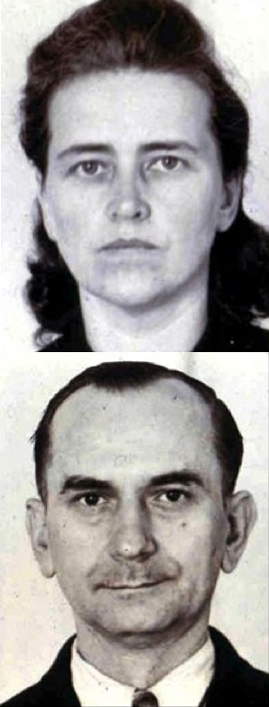
Peter Sutcliffe, also known as the Yorkshire Ripper, was the name on a list of 268,000 suspects generated by this investigation in the late 1970s. But how were the team investigating these crimes meant to cope with such an overload of information? These are the fundamental problems that geographic profiling is trying to solve.
How exactly does geographic profiling work? This article will introduce you to the fundamental ideas behind the subject. We will also look at the various applications, just like the Yorkshire Ripper case, along the way. These examples aren’t just in criminology though. The applications span ecology and epidemiology too!
The first model
Geographic profiling uses the spatial relationship between crimes to try and find the most likely area in which a criminal is based; this can be a home, a work place or even a local pub. Collectively we refer to these as anchor points. The pioneer of the subject, Kim Rossmo, once a detective inspector but now director of geospatial intelligence/investigation at Texas State University, created the criminal geographic targeting model in his thesis in 1987. The criminal geographic targeting model aims to do exactly what we struggled with at the beginning of this article: prioritise a huge list of suspects.

A gridded-up map. Alistair Marshall, CC BY 2.0
It starts by breaking up your map, populated with crime, into a grid, much like on the left. We assume that each crime that occurs, does so independently from every other. We then score each grid cell; the one with the highest score is likeliest to contain the criminal’s potential anchor point.
How do we calculate this score? An important factor is the distance between crimes and anchor points. We choose to use the Manhattan metric as our measure of distance. In this metric, the distance between points $\boldsymbol{a}$ and $\boldsymbol{b}$ is the sum of the horizontal and vertical changes in distance. This is written as:
$$d(\boldsymbol{a},\boldsymbol{b}) = \lvert x_a-x_b \rvert + \lvert y_a-y_b\rvert, \qquad \boldsymbol{a} = (x_a, y_a), \quad \boldsymbol{b} = (x_b, y_b).$$
The Manhattan metric is so-called because it resembles the distance you have to travel to get between two points in a gridded city like Manhattan.
This is the most suitable metric for our work, but it’s worth noting there are more that can be used (depending on the system you’re studying). Now we could just start searching at the spatial mean of our crimes and work radially outward from that point, however one rogue crime occurring far away from the rest could easily throw a spanner in the works. Instead we use something called a buffer/distance decay function.

$$ f(d) =
\begin{cases}
\dfrac{k}{d^{h}}, & d > B \\
\dfrac{kB^{g-h}}{(2B-d)^g}, & d\leq B\\
\end{cases}$$
A criminal isn’t likely to commit a crime close to an anchor point, out of fear of being recognised, so we place a buffer around it. In addition, to commit a crime far away from home is a lot of hassle, so the chance of a crime decays as we move away from the anchor point. This is why our buffer/decay function looks a bit like a cross-section of a volcano. The explicit function, $f(d)$, is written on the right, where $k$ is constant, $B$ is the buffer zone radius and $g$ and $h$ are values describing the criminal’s attributes, eg what mode of travel they use. With our distance metric, $d$, and buffer/decay function, $f$, we are now able to compute a score for each grid cell.
For $n$ crimes, the score we give to cell $\boldsymbol{p}$ is
$$ S(\boldsymbol{p}) = \sum_{i=1}^{n}f(d(\boldsymbol{p}, \boldsymbol{c}_i)), $$
where $\boldsymbol{c}_i$ is the location of crime $i$. So finally we have a score for each grid cell and we can prioritise our list!

An example of the geographic profile created using the criminal geographic targeting model
Plotting these scores on the $z$-axis produces a mountain range of values, like on the right. We can now prioritise by checking residencies at the peak of this mountain range and working our way down. Notice the collection of peaks around a particular area: this gives us an indication that perhaps the criminal uses more than one anchor point.
An important question: how can we be sure this even works? Does it really identify anchor points efficiently? What do we even mean by “efficient”? This is answered with a quantity called the hit score. This is
$$\text{hit score} = \frac{\text{number of grid cells searched before finding the criminal}}{\text{total number of grid cells}}. $$
So ironically, the lower our hit score, the better our model performs. This is sensible, since we want to search as little space as possible to catch our criminal.
The Gestapo case
Otto and Elise Hampel distributed hundreds of anti-Nazi postcards during the second world war. The Gestapo’s intuition on where the Hampel duo might live was based on themes almost exactly the same as geographic profiling. Inspired by a classic German novel, Alone in Berlin, our group revisited the Gestapo investigation and published our findings in a journal that is so highly classified we are not able to read it.
By analysing the drop-sites of the postcards and letters we were able to show that geographic profiling successfully prioritises the area where the Hampels lived in Berlin. Crucially, this study actually showed the importance of analysing minor terrorism related or subversive acts to identify terrorist bases before more serious crimes occur.
A statistical approach
The criminal geographic targeting model is an incredibly useful tool and is used to this day by the CIA, the Metropolitan Police and even the Canadian Mounted Police. Mike O’Leary, professor at Towson University, Maryland asked why the criminal geographic targeting model only produces a score, when we require a probability. So he developed a way of using geographic profiling under the laws of Bayesian probability.

Bayes’ rule is better in neon. Image: Wikimedia Commons user Mattbuck, CC BY-SA 3.0
O’Leary uses Bayes’ rule as seen on the right. How do we apply it to criminology? We want to know: what is the probability that an offender is based at an anchor point given the crimes they have committed? Using Bayes’ rule, instead we pretend we know where the anchor point is and ask; what is the probability of the crimes occurring given our anchor point? We use the formulation
$$\Pr(\boldsymbol{c}_1, \boldsymbol{c}_2, \boldsymbol{c}_3, \boldsymbol{c}_4\text{…}\;|\;\boldsymbol{p})\; = \;\prod_{i=1}^{n}\Pr(\boldsymbol{c}_i\;|\;\boldsymbol{p}),$$
where the equality derives from the assumption of independent crimes.
Below, we can see a comparison between Rossmo’s criminal geographic targeting model and O’Leary’s simple Bayesian model. The problem with O’Leary’s model is he assumes that a criminal only has one anchor point. Unfortunately this is rarely the case. As we mentioned earlier, an anchor point could be a home, a workplace, a local pub or even all of the above. So we obtain a probability surface, but we only consider one anchor point. The criminal geographic targeting model entertains the idea that multiple anchor points exist, but doesn’t give us an explicit probability. What we really need is a way of combining both methods. Does such a method exist?
 (a) The criminal geographic targetting model |
 (b) The simple Bayesian model |
Examples of the geographic profiles created using the criminal geographic targeting and simple Bayesian models
The elusive tarsiers

Image: Callum Pearson
Using only the GPS location of tarsier vocalisations as input into the geographic profiling model we were able to identify the location of tarsier sleeping trees. The model found 10 of the 26 known sleeping sites by searching less than 5% of the total area (3.4 km$^2$). In addition, the model located all but one of the sleeping sites by searching less than 15% of the area. The results strongly suggest that this technique can be successfully applied to locating nests, dens or roosts of elusive animals, and as such be further used within ecological research.
The best of both worlds
The Dirichlet process mixture model is the best of both the criminal geographic targeting and the simple Bayesian models. So far we’ve only stated that we’re either working with one anchor point, or many. The beauty of the Dirichlet process mixture model is that we don’t need to specify the number of anchor points we are searching for. Instead, there is always some non-zero probability that each crime comes from a separate anchor point. So multiple anchor points can be identified while using a probabilistic framework. Introducing multiple anchor points is challenging since we need to know:
- How are all the crimes clustered together?
- In each cluster of crimes, where is the anchor point?
Actually, what would be really useful is if we knew the answer to just one of these questions. If we knew how the crimes were clustered, finding the anchor points is easy (we use the simple Bayesian model to find the source in each cluster). But also, if we knew where the anchor points were, allocating crimes to clusters is easy (and of course we know where our criminal lives!). The solution to this problem is to use something called a Gibbs sampler. We use a Gibbs sampler in cases where we want to sample a set of events that are conditional on one another. In our case, anchor point locations depend on the clustering of crimes, but the clustering of crimes also depends on the anchor point locations. The steps the Gibbs sampler will take are:
- Randomly assign each crime an anchor point (even though we don’t yet know where the anchor points are).
- Find each anchor point by using the simple Bayesian model on each assignment.
- Throw out the assignments of crimes to anchor points and now re-assign crimes but using the locations found in previous step. Throw out the old anchor point locations and find new ones using this new assignment.
- Repeat steps 3 and 4 many, many times.
This produces a new profile like on the right below. We can now compare this to our other two models on the left. We can see the Dirichlet process mixture model displays fewer peaks than the criminal geographic targeting model, but that these peaks are tighter. This in turn will reduce the hit score of our search.
 (a) The criminal geographic targetting model |
 (b) The simple Bayesian model |
 (c) The Dirichlet process mixture model |
A comparison of the three main geographic profiling models
The malaria case

Water bodies with mosquito larvae. Image: © OpenStreetMap contributors. Cartography CC BY-SA 2.0
Throughout history, infectious diseases have been a major cause of death, with three in particular (malaria, HIV and tuberculosis) accounting for 3.9 million deaths a year. Targeted interventions are crucial in the fight against infectious diseases as they are more efficient and, importantly, more cost effective. They are even more crucial when the transmission rate is strongly dependent on particular locations. For example, we were tasked with finding the source(s) of malaria outbreaks in Cairo by considering the breeding site locations of mosquitos.
All accessible water bodies within the study area were recorded between April and September 2005, and 59 of these were harbouring at least one mosquito larva. Of these 59 sites, seven tested positive for An. sergentii, well-established as the most dangerous malaria vector in Egypt. Using only the spatial locations of 139 disease case locations as input into the model, we were able to rank six of these seven sites in the top 2% of the geoprofile.
Applying the method
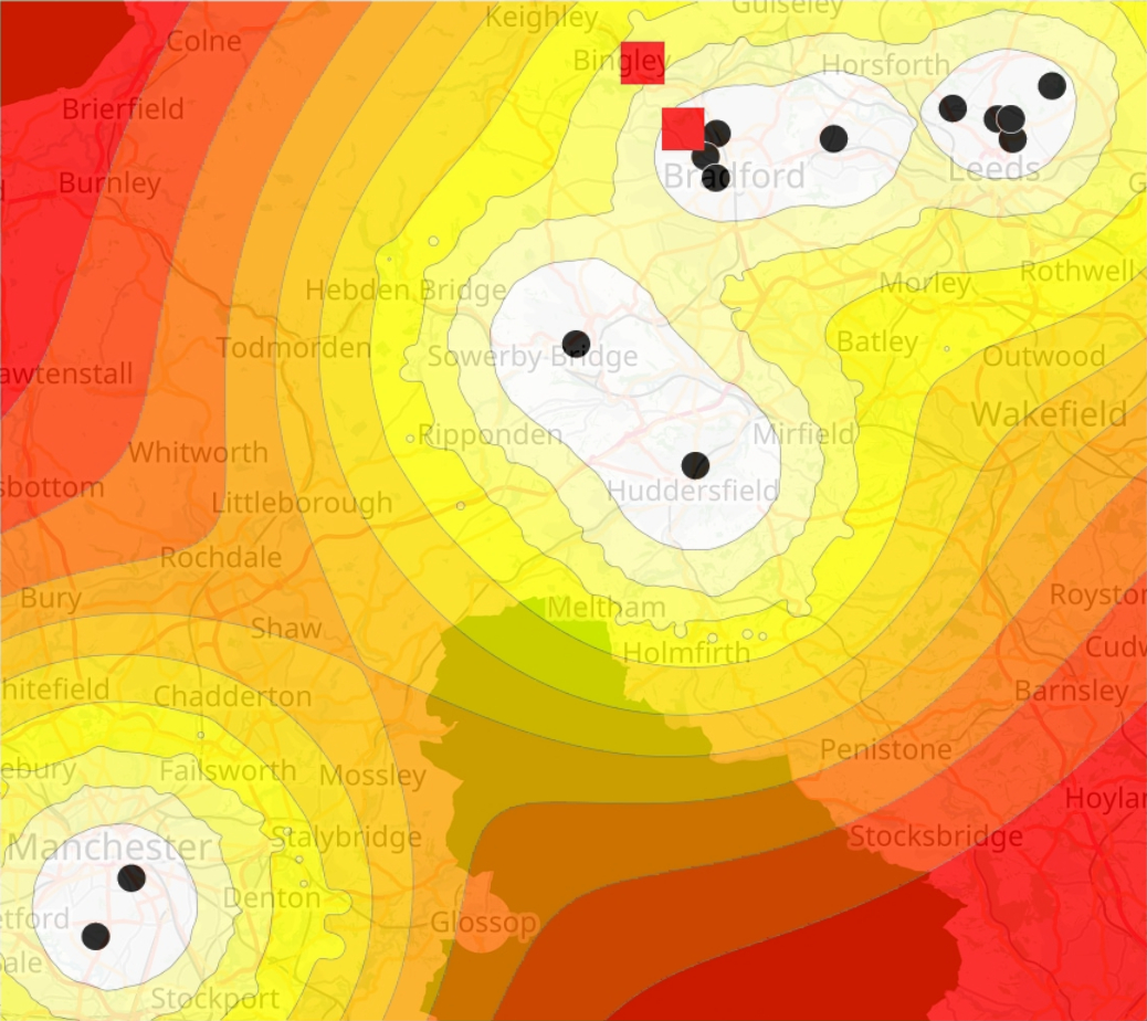
The geoprofile associated with the Yorkshire Ripper body dump sites (black dots). The anchor points of Peter Sutcliffe are labelled as red squares. Image: © OpenStreetMap contributors. Cartography CC BY-SA 2.0
We’ve done it! We now have a robust method for searching for our criminal. A list of 268,000 suspects is no longer so intimidating. Without this technique in 1975-1981, however, there was a lot more work for the team investigating the Yorkshire Ripper case. On top of a huge list of suspects, 27,000 houses were visited and 31,000 statements were taken during the investigation.
If we apply our model to the crime sites we were given at the start of this article, we produce the contour map on the right. In this case the areas in white describe the highest points on our probability surface, whilst areas in red describe the lowest. In addition to the contours, we also see two red squares right at the top of the map. These are the two homes Peter Sutcliffe resided at during the period of his crimes. The hit scores for his two residences are 24% and 5% respectively. So by searching only 24% of our total search area, we’ve managed to find both residences. This is far better than a random search which would find them after searching, on average, 50% of our area.
Peter Sutcliffe’s homes are clearly marked on this map but we must remember an important point about geographic profiling: that it is not an ‘X marks the spot’ kind of model, but rather a method of prioritisation.
Investigating an old case

Dramatic scenes covered the newspaper front pages, such as this from 1888. Image: The Illustrated Police News
We can’t talk about the Yorkshire Ripper without mentioning the notorious 1888 London serial killer, Jack the Ripper. The five locations around Whitechapel where bodies were dumped were studied using geographic profiling to try and gain a better idea of where Jack the Ripper may have lived.
The map overleaf shows us the associated geoprofile, with Jack’s suspected anchor point obtaining a hit score between 10-20%, much better than a non-prioritised search!
This is just one example of many cases where we can utilise our new model to study cases from the past where such tools were not available.
Geographic profiling began in criminology, but now spans ecology (catching invasive species) and epidemiology (identifying sources of infectious disease) too. This means saving a hefty chunk of time and money, as well as developing prevention strategies to minimise any negative impacts these problems may cause.
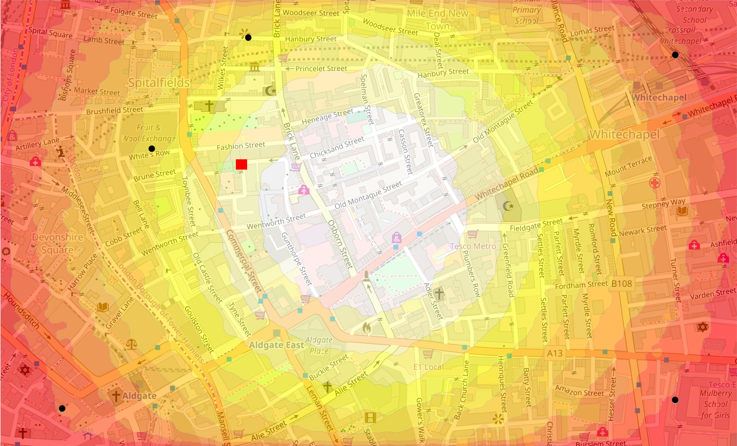
The geoprofile associated with the body dump sites (black dots) of Jack the Ripper. Jack’s anchor point (the red square) is suspected to be around Flower and Dean Street. Image: © OpenStreetMap contributors. Cartography CC BY-SA 2.0
More from Chalkdust

In conversation with Cédric Villani
We feel underdressed for Breakfast at Villani's
Cardioids in coffee cups
Staring at your coffee, you wonder whether the light reflecting in cup really is a cardioid curve...
Mathematics for the three-fingered mathematician
Robert J Low flips one upside down.
The mathematics of Maryam Mirzakhani
We take a proper look at her mathematical accomplishments
Biography of Sophie Bryant
A biography of Sophie Bryant
Roots: Blaise Pascal
Blaise Pascal was driven to begin the mechanisation of mathematics by his father's struggles with an accounts book in 17th century France.
Pingback: Students co-author magazine article - The London NERC DTP | The London NERC DTP