
High-speed internet and digital storage get cheaper, but the challenge of sharing large files is one that anybody who spends their time working on computers faces. Digital images in particular can be a pain if they lead to long loading times and high server costs. If you have ever seen an image on the internet, then you have certainly encountered the JPEG format because it has been the web standard for almost 30 years. I am sure, however, that you have never heard of its potential successor, JPEG2000, even though it recently celebrated its 20th anniversary. If so, then that is unfortunate because it produces much better results than its predecessor.
Same principle but different outcome
The best way to understand why different formats give very different outcomes is to look at a specific example. I have compressed a picture of myself using JPEG and JPEG2000. In both cases I sacrifice image quality in favour of space savings, which leads to errors in the resulting image. With JPEG, an image usually starts to become blurry as soon as it is compressed. You’ve probably noticed it with images on the web. Additionally, there can also be a colour loss so the image has a duller appearance overall. In my picture, the most obvious thing to suffer is that smooth colour gradients have been replaced by monochrome areas which make it appear like a picture inside a colour-by-numbers book. We can see some distinct patches of grey on the left wall for example. With JPEG2000, on the other hand, image quality usually only starts to noticeably decrease after extensive compression. As you can see, the image on the right still looks relatively unchanged.

Image of the author compressed using JPEG and JPEG2000. Note that compression does not
make the image smaller, they have been scaled down here to make room for the details.
The differences between the two compressions are the result of the underlying mathematical procedures. JPEG uses the discrete cosine transform, whereas JPEG2000 uses the discrete wavelet transform. ‘Discrete’ refers to the fact that computers only deal with information in chunks called bits while ‘cosine’ and ‘wavelet’ stand for the functions that are used to sample the image. The wavelet transform is so-called because the function it uses looks like small waves when graphed:
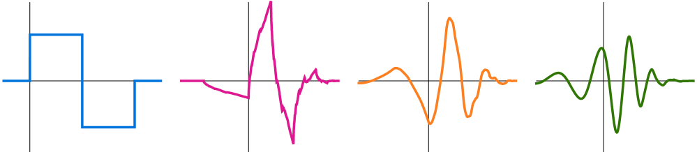
Left to right: Daubechies wavelets of order 1, 2, 4 and 8.
The one on the left is also called a Haar wavelet. We will encounter it in matrix form later when I explain how JPEG2000 works. I want to show you how it can save more storage space while still delivering better looking images.
From analogue to digital
When we transform an analogue image to a digital image, we view it as a grid of blocks with a predetermined size. We call these blocks pixels, which stands for ‘picture elements’, and assign each of them a number corresponding to their colour. And just like that, we have transformed our image with coloured blocks into a matrix with numbers. The entries in a monochrome image matrix are brightness values from 0 for black to 255 for white. Colour images require a few additional parameters, but the important thing is that the file size of a digital image depends on the number of pixels and the size of the colour scale.
Sometimes a low resolution is quite sufficient since our human eyes cannot detect any difference from the original once we view an image at a certain distance. That is why JPEG is ideal for small images such as thumbnails where resolution does not matter as long as you can recognise what is depicted. However, when the image is larger, you have already witnessed some potential side effects of the compression with JPEG in my sample picture. We can check the occurrence of these so-called artefacts with suitable image galleries. Think of these as collections of images with problematic patterns that are susceptible to various defects. The image ‘Barbara’ below, for example, is perfectly suited for the detection of block artefacts due to the rapid sequences of light-dark areas it contains.

The test image ‘Barbara’, with a detail compressed using JPEG and JPEG2000. Image: Fabien Petitcolas, public domain.
The principle of compression is that unnecessary information must be located and thrown away. We will use some elegant mathematics to change the values in our image matrix so that this redundant information becomes visible. We try to find as many entries as possible according to specific criteria and set them to zero. The result is an approximation that is then efficiently coded. I will not go into detail here, but the general idea of this last step is as follows: since each digital colour value is saved as a list of ones and zeros, we look for values that appear with higher frequency and assign them abbreviated labels instead to save space. In the case of the value zero, we could write it as just 0 instead of its complete 8-bit binary notation 00000000. If we have lots of black areas in our image we can use this shorter notation to save space. This, however, is not exactly the algorithm used in image compression; look up ‘Huffman encoding’ if you are interested.
Let’s look at the numbers

Computers store data in bits containing the value 0 or 1. Image: Flickr user Christiaan Colen, CC BY-SA 2.0
The memory requirement of a digital image is measured in bits. One bit corresponds to the smallest possible digital storage unit that takes either the value 0 or 1. We can use this to work out the compression rate by dividing the number of bits for the compressed image by the number for the original. If the fraction is close to zero, this means that we saved a lot of space and vice versa. My original image is 2976 $\times$ 3968 $\approx$ 12,000,000 pixels large and requires about 12,500,000 bytes of storage space. To convert bytes into bits, we multiply by eight (1 byte $=$ 8 bits), which gives us 100,000,000 bits. The JPEG file requires about 2,220,000 bits, and the JPEG2000 file only about 800,000 bits. With this, we get compression rates of approximately 0.02 for JPEG and 0.01 for JPEG2000. Both of my compressions are quite good since each requires only a tiny percentage of the original memory space. We can see, however, that the JPEG file suffers from a noticeable drop in image quality. The JPEG2000 version of my picture, on the other hand, looks relatively unchanged while still being more efficient with only about 36% the size of the JPEG file. Let’s find out how this is possible.
As a rule of thumb: JPEG files with compression rates below 0.25 tend to experience severe quality losses. The discrete cosine transformation used by JPEG represents the values of pixel blocks (usually $8 \times 8$ pixels in size) as combinations of cosine oscillations and makes use of orthographic projections to replace them with simplified versions. Imagine it like this: the transformation has a set of versatile building blocks like Lego bricks that we can combine to build any image. If you restrict yourself to use only a few different types of Lego bricks, you can still approximate the image, but the more you limit your options, the cruder the approximation will look as you can see in the ‘Barbara’ image. The reason why the corners and edges of block artefacts become more apparent at higher compression rates is that the available options are not versatile enough to create a convincing approximation.
The discrete wavelet transform
To figure out how JPEG2000 works, we start with a simple task: we count the number of passengers at a train station throughout an eight-hour shift which gives us a list of numbers: $($206, 306, 59, 69, 16, 16, 5, 3$)$. Let’s suppose we want to send this information to someone, but we need to compress it first to save space (this is just an example—in practical applications, compression becomes necessary only when you send a lot more data). How should we choose the numbers we send? Assuming we are satisfied with a rough count, a viable option could be to round the numbers to their nearest multiple of ten: $(200, 300, 60, 70, 20, 20, 10, 0),$ but there is a better way.
Another possibility is to form averages of the four consecutive pairs: $(256, 64, 16, 4)$. Doing this requires only four values, but nobody can decrypt the original numbers without additional information. Fortunately, we still have four empty slots left in our list. We can choose another number for each of the four pairs which allows us to decrypt the input from the average and tells us something else about the numbers.
The linear transform $\widetilde{\boldsymbol{\mathsf{W}}}$ generates both the mean of a number pair $ (a, b) $ and the absolute difference between the mean and either of the two numbers $\widetilde{\boldsymbol{\mathsf{W}}}: (a, b) \to ((b+a)/2, \left|b-a\right|/2)$. The four additional numbers are now $(50, 5, 0, 1)$. This process is easily reversible: we get our starting numbers by adding and subtracting the differences from the corresponding means. More revealing, however, is that these differences measure the distribution of the original numbers. A high value means that the original number pair was far apart and a low value means they were close together.
The discrete wavelet transform used by JPEG2000 takes advantage of the fact that these differences capture the redundant information we can remove when we want to compress an image. As long as the values are smaller than a certain threshold which depends on the intended level of compression, we can set them to zero. In our example, the threshold could be 10, so the compressed differences are $(50, 0, 0, 0)$, and reversing the process gives us the list $(206, 306, 64, 64, 16, 16, 4, 4)$. The result is very similar to the original list even though we have simplified most of the differences. For images, this means that we match neighbouring pixels with a similar colour by setting their difference to zero, which we can then efficiently code to save space.
When doing this with a computer, we can use matrix algebra to simplify the calculations. If we have a list of numbers, that is, a vector $\boldsymbol{\mathsf{v}}$ of even length, we can write the transformed vector: $\boldsymbol{\mathsf{w}}=\widetilde{\boldsymbol{\mathsf{W}}}\boldsymbol{\mathsf{v}}$. If we have two or four data points, for example, the transformation is a $2\times2$ or $4\times4$ matrix:
\[\widetilde{\boldsymbol{\mathsf{W}}}_2 = \begin{pmatrix} 1/2 & 1/2 \\ -1/2 & 1/2 \end{pmatrix},\quad \widetilde{\boldsymbol{\mathsf{W}}}_4 = \begin{pmatrix} 1/2 & 1/2 & 0 & 0 \\ 0 & 0 & 1/2 & 1/2 \\ -1/2 & 1/2 & 0 & 0 \\ 0 & 0 & -1/2 & 1/2 \end{pmatrix}.\]
We can also reverse the process by using the rules for matrix multiplication: $\widetilde{\boldsymbol{\mathsf{W}}}^{-1}\boldsymbol{\mathsf{w}} = \boldsymbol{\mathsf{v}}$. The discrete Haar wavelet transform (HWT) for an input vector of length $N = 2k$ (with $k \in \mathbb{N}$) is defined as $\boldsymbol{\mathsf{W}}_N = \sqrt{2} \widetilde{\boldsymbol{\mathsf{W}}}_N$. The factor $\sqrt{2}$ is added to make the matrix orthogonal (this simplifies calculating the reverse transformation) but you only need to pay attention to $\widetilde{\boldsymbol{\mathsf{W}}}_N$ to understand what is going on. It is great for illustrating how wavelet transforms work since it is relatively simple. The first $ N/2 $ rows of the result of the Haar wavelet transform contain the averages of the number pairs and the remaining $ N/2 $ rows their respective differences.
Transforming an image
Now we can apply the transform to any $ N \times M$ pixel image matrix $\boldsymbol{\mathsf{B}}$. Since an image is a two-dimensional array of numbers, we want to apply the transform both vertically and horizontally. More precisely, instead of a single list with $ N $ elements, we now transform $M$ lists with $N$ elements each. The result is also an $ N \times M$ matrix divided into two halves: the upper average block and the lower difference block. You can follow the process in the picture below, starting from the left. This first step corresponds to the one-dimensional Haar wavelet transform (1D-HWT) because we only transformed the matrix vertically. To do the same with the rows and thus transform the image completely, we use the rules for matrix multiplication and get $\widetilde{\boldsymbol{\mathsf{B}}} = \boldsymbol{\mathsf{W}}_M \boldsymbol{\mathsf{B}} \boldsymbol{\mathsf{W}}_N^{-1} $. The result of the complete, or two-dimensional, Haar wavelet transform (2D-HWT) is again an $N \times M$ matrix divided into four blocks. On the right, you can see that most of the intensities are contained in the upper left block while the remaining blocks are mostly black because they include mainly the sought-after values close to zero that we can round down to save space.

Left: 1D-HWT; right: 2D-HWT.
Let’s take a closer look at their composition. The upper left block is composed of averages of the rows and columns and looks like a smaller version of the image. The lower left block reveals information about the horizontal details, while the upper right block contains the vertical ones. Lastly, the lower right block is made up of differences of the rows and columns and corresponds to the diagonal details. Notice that the three detail blocks only have high values at locations with a drastic change in brightness which is why we can see the outlines of the images there.
Repetition and reversion

2D-HWT applied twice.
In practice, we repeat this process as often as possible to increase the saving potential even further by reapplying it to the previous approximation in the top left corner. Each time the process is repeated, the block containing the averages becomes more compact. For an $N \times M$ pixel image matrix, $ p $ iterations of the Haar wavelet transform can be performed if both $ N $ and $ M $ are divisible by $ 2^p $. To restore the original image, we need to apply the inverse transform to the approximation as many times as needed. You can think of it as sharpening the image because the approximation gets more and more detailed with each iteration we undo. Of course, this is only completely possible if we compressed the file without discarding any data. When we reverse the process after rounding values to zero, we end up with an approximation of the original image which is our compressed version.
Wrapping things up
Now we know why the results with JPEG2000 are not only more efficient but also better looking. It transforms the image as a whole instead of small $8 \times 8$ chunks. You might ask: “Why is it not being used by the general public despite faring so much better than JPEG?” The answer could be that it takes a lot of time and effort to change the standards for such a large-scale application like image processing. Another hurdle is that the old format still seems to be sufficient. JPEG2000 has found its home in fields like medical scanning, but we probably will not see it taking over anytime soon. Today there are also some new contenders like WebP and AVIF that may supersede JPEG2000 anyway. Increasing demand for less data traffic due to environmental concerns might lead to a rise in popularity for alternative formats. I urge everybody interested in image processing to check out JPEG2000 and compress a few image files for themselves.
More from Chalkdust

In conversation with Ulrike Tillmann
Sophie Maclean and David Sheard speak to a very top(olog)ical mathematician!
On conditional probability: Cards, Covid, and Crazy Rich Asians
Madeleine Hall explores the sometimes counterintuitive consequences of conditional probability to our everyday lives.
The maths of Mafia
Sophie explores the fascinating mathematics behind the games Mafia and Among Us.
Who is the best England manager?
Paddy Moore levels the score
How to be the least popular American president
Francisco Berkemeier takes a look at the mathematics behind elections, and the Electoral College, in the United States of America.
On the cover: cellular automata
Discover the meaning of the coloured squares on the cover of issue 13