
You have to go a long way to beat the magnetic pendulum for demonstrating the deep and profound nature of physics. One is pictured on the right. On the face of it, a swinging bob seems simple enough to understand. But as is so often the case, simplicity is masking complexity and the motion possesses an almost magical quality. Here, we will take a glimpse into just how unpredictable the predictable can really be.
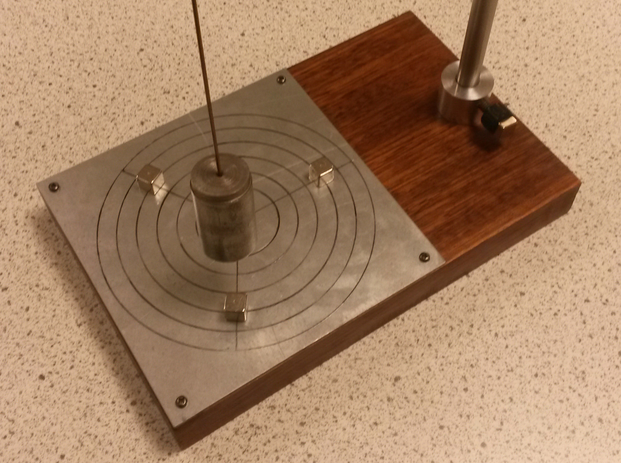
The magnetic pendulum: it comprises a bob with a small magnet suspended by a string above a base plane that contains similar magnets arranged with opposite poles to ensure attraction.
Pull the pendulum back some distance in any direction, let it go, and prepare to be mesmerised by the way it darts back and forth in an erratic and seemingly random way. The bob is drawn simultaneously to all three base-plane magnets until, finally, it tends towards a precarious state of rest above one of them. Playing like this, it does not take long to become convinced of two immutable facts. Firstly, one can never know beforehand over which magnet the bob will stop. Secondly, and perhaps more subtly, the motion is not reproducible. No matter how hard one tries to replicate the initial displacement, the bob never follows the same winding path twice and the magnet that ultimately `wins’ seems to be governed by chance. How can we possibly find such randomness in a tabletop toy?
Of course, the bob is not moving randomly at all and we are at best starting it off each time from only roughly the same initial conditions. Its motion is prescribed by purely deterministic equations, a combination of classical mechanics and electromagnetics, and at that level there is no randomness. Were we able to release the bob from exactly the same starting position each time, the subsequent motions would all be identical and they would always stop at the same place. No uncertainty. No unpredictability. No endless fascination!
Since our first pull can never be repeated with infinite precision, what we are seeing is sensitive dependence on initial conditions or, more colloquially, the butterfly effect. Any change in input—any, no matter how imperceptibly small—can have a dramatic impact on output. That intriguing phenomenon turns out to be far more widespread and pervasive than one might first imagine. Moreover, it provides our working definition of chaos and crystallises what we mean by saying ”a system is chaotic”. In this article, we will start to explore how the magnetic pendulum embodies chaos in the scientific (rather than the everyday) sense.
A phenomenological model
It is not too difficult to devise a model that exhibits all the key qualitative features of the magnetic pendulum. Our approach is a phenomenological one, meaning that we are aiming to capture the essence of the motion using intuitive physical ideas rather than focusing on all the mathematical minutiae. A relatively easy way forward is to consider looking down on the pendulum from a plan view (see figure below). The bob’s trajectory in the three-dimensional space is projected downwards onto the horizontal base plane, and the origin of the $(x,y)$ coordinates is fixed at the centre of an equilateral triangle. The magnets are subsequently located at vertices $ \mathbf{X_1} $ , $ \mathbf{X_2} $ , and $ \mathbf{X_3} $, all of which lie along the circumference of a circle with a radius taken to be the unit length.
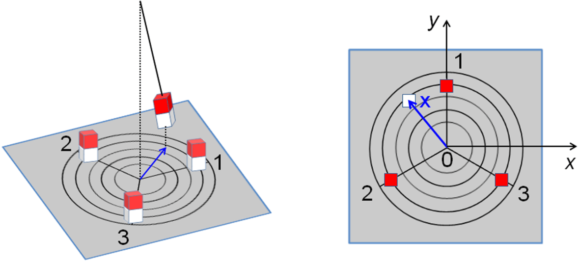
Left: Schematic diagram of the magnetic pendulum. Right: Projecting the position of the bob (white square at position $ \mathbf{x} $ ) onto the horizontal $(x,y)$ plane. The base-plane magnets (red squares 1, 2, and 3) are positioned at the vertices of an equilateral triangle.
The position vector of the bob may be represented by $\mathbf{x}(t)$ at time $t$. To account for gravity, it is sufficient for our purposes to consider a restoring force $\mathbf{F}_\text{grav} \propto -\mathbf{x}$ whose influence, due to the minus sign, always acts to pull the bob towards the origin $\mathbf{x} = \mathbf{0}$ (the constant of proportionality is set equal to 1, just to keep things simple). Dissipation might be introduced by way of the standard velocity-dependent damping force familiar from textbook physics. Here, we use $\mathbf{F}_{\text{losses}} = -b\mathbf{u}$, where $\mathbf{u} \equiv \mathrm{d}\mathbf{x}/\mathrm{d}t$. For some constant $b > 0$, the effect of $\mathbf{F}_{\text{losses}}$ is to drain kinetic energy from the motion through air resistance at low speeds. Finally, we must look to include the attractive forces due to the base-plane magnets. It is tempting to reach immediately for the inverse-square rule familiar from Coulomb’s law of electrostatics and Newton’s law of universal gravitation. We instead opt for a $1/\text{distance}^4$ rule as this form tends to describe the forces exchanged by magnetic dipoles.
Since Newton’s second law of motion equates mass $\times$ acceleration to the combined forces of gravity, magnetism, and damping, we can write down a governing equation of the form
\begin{equation}
\frac{\mathrm{d}^2\mathbf{x}}{\mathrm{d}t^{\hspace{0.5mm}2}} + b\frac{\mathrm{d}\mathbf{x}}{\mathrm{d}t} + \mathbf{x} = \sum_{n=1}^3\frac{\mathbf{X}_n – \mathbf{x}}{\left(|\mathbf{X}_n – \mathbf{x}|^2+h^2\right)^{5/2}}.
\end{equation}
Pythagoras’s theorem has been deployed here, and so each contribution in the summation on the right-hand side of (1) corresponds to a `distance/distance$^5 =$ 1/distance$^4$’ type of term. An additional parameter, $h^2$, has also appeared. Its role is to suppress unphysical (that is, infinite!) accelerations that would otherwise result whenever $\mathbf{x}$ approaches $\mathbf{X}_n$. We then interpret $h$ as being related to the average height of the bob above the base plane.
The equilibrium points are defined to be those positions $\mathbf{x}=\mathbf{x}_\text{eq}$ that are unchanging in time. Since the velocity and acceleration of the bob must be zero at those points (hence satisfying $\mathrm{d}\mathbf{x}_\text{eq}/\mathrm{d}t = \mathbf{0}$ and $\mathrm{d}^2\mathbf{x}_\text{eq}/\mathrm{d}t^{\hspace{0.5mm}2} = \mathbf{0}$, respectively), it follows from (1) that
\begin{equation}
\mathbf{x}_{\text{eq}} = \sum_{n=1}^3\frac{\mathbf{X}_n – \mathbf{x}_{\text{eq}}}{\left(|\mathbf{X}_n – \mathbf{x}_{\text{eq}}|^2+h^2\right)^{5/2}}.
\end{equation}
After playing with the pendulum and noting the positions where the bob tends to stop, we might reasonably expect to find maybe three or at most four solutions (with $\mathbf{x}_{\text{eq}} = \mathbf{0}$ being the origin). It is worth mentioning that the nontrivial roots of (2) do not occur at $\mathbf{x}_{\text{eq}} = \mathbf{X}_n$, as one might initially suspect. Instead, they lie at the same angular positions as $\mathbf{X}_n$ (as symmetry demands) but at a radial distance $|\mathbf{x}_\text{eq}|$ that is slightly less than unit length. At these positions, the competing pulls from gravity and magnetism are perfectly balanced.
Equation (1) does a surprisingly good job at mimicking the unpredictability so readily seen in experimental demonstrations; the left-hand side is just the damped harmonic oscillator problem from mechanics while the right-hand side sums over the pairwise magnetic-dipole interactions. On the one hand, any urges to seek analytical solutions should be kept in check. Even this stripped-down toy model confronts us with a formidable mathematical beast living in a four-dimensional realm whose axes are $(x,y,u_x,u_y)$. On the other hand, computing a numerical solution can be relatively quick and easy for given initial conditions, say $\mathbf{x}(0) = \mathbf{x}_0$ and $\mathbf{u}(0) = \mathbf{0}$.
Basins of attraction
Physically, we anticipate that the bob will almost inevitably come to rest at one of the non-trivial equilibrium points $\mathbf{x}_\text{eq}$ [cf. (2)] as $t\rightarrow\infty$. Those special points can be thought of as positions in the $(x,y)$ plane that attract the trajectory, and accordingly they are often referred to as fixed-point attractors. The idea now is to use a computer to carry out a systematic set of simulations, recording which magnet `wins’ (interpreted as the output) as we vary the starting point $\mathbf{x}_0$ (taken to be the input). By associating the outcome of each computation with a colour (eg red for magnet 1, white for magnet 2, and black for magnet 3), we can overlay the output on top of the input $(x_0,y_0)$ plane to produce a kind of abstract map. The set of all initial conditions lying in the red region is the basin of attraction for magnet 1—that is, any $\mathbf{x}_0$ lying on a red point will always end up at magnet 1 (and similar for the other colours and magnets), though the colour itself gives no information about the path taken by the bob to arrive at that point.
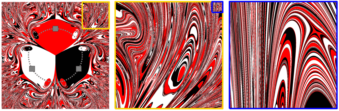
Figure 1. Basins of attraction for the magnetic pendulum with $b = 0.1$ and $h^2 = 1/4$. In the first pane, the grey squares denote the position of the base-plane magnets and the dotted grey line is a circle with radius equal to the unit length. The second and third panes show successive magnifications.
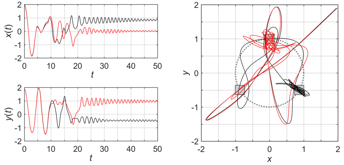
Figure 2. An illustration of FSS in the magnetic pendulum. Two initial conditions that are arbitrarily close together can give rise to subsequent trajectories that will start to move away from one another after a finite amount of time. The red path ends at magnet 1, while the black path ends at magnet 3.
Using this recipe, we discover a rather striking pattern (see fig. 1). Regions around the origin appear relatively simple. There are large single-colour lobes which indicate that variations in $\mathbf{x}_0$ tend to have little impact on which magnet wins. Further out beyond the unit circle, there is much greater complexity and all three colours are intertwined in a beautifully complicated way. In those regions, the pendulum is extremely sensitive to changes in $\mathbf{x}_0$. Successive zooming-in suggests the intertwining survives down to smaller and smaller length-scales. That feature—proportional levels of pattern detail persisting under arbitrary magnifications—is a defining characteristic of a fractal. A less obvious but equally fascinating property relates to the nature of the boundary separating two differently-coloured regions. We typically cannot cross from a region of red to an adjacent region of black without touching the white (similar is true for other permutations of colours). This situation is reminiscent of the delightfully strange Wada property from the field of topology.
Final state sensitivity

Figure 3. Variation of the basins of attraction for the magnetic pendulum as damping is increased. The second and third columns show successive magnifications. Other parameters and domains of the $(x_0,y_0)$ plane are the same as those in fig. 1.
The basins of attraction have three-fold rotation symmetry about the origin, which is a consequence of the equilateral-triangle arrangement of magnets and the initial condition $\mathbf{u}(0) = \textbf{0}$. Their details also depend crucially on system parameters. One might consider what happens, for instance, when the level of damping is increased (see figure to the right) through $b=0.125$ (first row), $b=0.150$ (second row), $b=0.175$ (third row), and $b=0.200$ (bottom row). The pattern becomes less complex and, accordingly, the pendulum less sensitive to small fluctuations in $\mathbf{x}_0$. However, their key features remain intact: the persistence of self-similar structure (fractality) and complex boundaries that tend to involve all three colours. The Wada-type property is still present in the right-hand column of the last two rows, but it is not obvious from these figures.
A helpful way to quantify just how strongly the long-term state of a system depends upon small fluctuations at its input is to estimate the fractal dimension $1 < D \leq 2$ of the basin boundaries. One selects a set of $N_\mathit{\Gamma}$ points in a domain $\mathit{\Gamma}$ of the $(x_0,y_0)$ plane and tests each of them in turn for the property of \textit{final-state sensitivity} (FSS) by considering a triplet of initial conditions: say $(x_0,y_0)$, $(x_0 + \epsilon,y_0)$, and $(x_0-\epsilon,y_0)$, where $0 < \epsilon \ll \mathcal{O}(1)$ can be interpreted as an error or as a limit to our experimental precision. When the winning magnet is the same for all three trajectories, then the final state is independent of $\epsilon$ and $(x_0,y_0)$ is, accordingly, free from FSS. Alternatively, think of $\epsilon$ as the radius of a small disc centred on $(x_0,y_0)$, somewhere within which the `true’ initial condition lies. FSS, as demonstrated in fig. 2, appears whenever that disc impinges on a basin boundary and thus overlaps more than one colour.
If the total number of points possessing FSS for a given $\epsilon$ is denoted by $N_\epsilon$, one finds that that $N_\epsilon/N_\mathit{\Gamma} \sim \epsilon^\alpha$. The parameter $\alpha \equiv 2 – D$ is known as the uncertainty exponent and it satisfies the inequality $0 \leq \alpha < 1$. Finally, we obtain the uncertainty dimension D, where
\begin{equation}
D = 2 – \frac{\mathrm{d}\log_{10}(N_\epsilon/N_\mathit{\Gamma})}{\mathrm{d}(\log_{10}\epsilon)}
\end{equation}
and a larger $D$ is indicative of increased susceptibility to initial fluctuations. The patterns shown in the middle panes of figs 1 and 3 turn out to have dimensions in the range $D\approx1.32$ (for $b = 0.1$) to $D\approx1.16$ (for $b = 0.2$). It follows that the basin boundaries for lightly-damped pendula tend to be associated with higher values of $D$. More generally, we now see a connection between the dimension of an abstract fractal pattern (which, crucially, need not be an integer such as 1 or 2) and the physical property of FSS.
Concluding remarks
In this article, we have started to unpick some of the intriguing behaviour exhibited by what is, in reality, a simple toy—one that never fails to capture the imagination of university students in lectures and Ucas applicants (and their parents alike!) at open days. The apparently erratic swinging and unknowable terminus of a bob are not quite so `random’ as one might first suppose from a few naïve observations. The essential ingredient giving rise to all this rich and diverse behaviour is the interplay between the three constituent feedback loops (here, due to gravity, dissipation, and magnetism).
Although we have considered the barest of bare-bones models (from pretending gravity provides a restoring force proportional to $-\mathbf{x}$, to suppressing the fully-vectorial character of magnetic interactions), the beautiful complexity of nature survives and we simply cannot get rid of it. That, it seems to us, is a mind-blowing conclusion!
More from Chalkdust

The Newton–Raphson fractal
James Christian and George Jensen zoom in, out, in, out, and tell us what it's really all about
Chaotic scattering: uncertainty and fractals from reflections
James M Christian reflects on chaos
In conversation with Eugenia Cheng
We chat to the author of the best-selling book How to Bake Pi and pioneer of maths on YouTube
Too good to be Truchet
Colin Beveridge looks at different designs for 2- and 3-dimensional tiles
Topological tic-tac-toe
Alex Bolton plays noughts and crosses on unusual surfaces
Somewhere over the critical line
Read about Maxamillion Polignac's adventures in a prime-hating world
Pingback: The Pendulum Fractal – Val's homepage