
Today at Chalkdust, we’re celebrating our love for mathematics, and what better way to do that than by analysing our heartbeats? The heart is composed of four main chambers: two atria at the top and two ventricles at the bottom. Apart from carrying our hopes and dreams, the heart’s main function is to pump blood around our body. This can be split into two different circuits, the first one is low-pressure (in blue below) and pumps blood from our body to our lungs to get oxygenated before coming back to the heart. The second is a high-pressure circuit (in red) which then pumps this oxygenated blood out of the aorta and to the rest of our body.

The sinoatrial node is highlighted in green, don’t worry about all the other labels.
We’ll take a step back from considering the blood flow and turn our attention to heartbeats. We know that there is a certain rhythm to heartbeats and a sequence in which the different chambers of the heart contract. During the heartbeat cycle, there are two equilibrium states, diastole (relaxed) and systole (contracted). I’ll be using these terms herein; an easy way to remember which is diastole is to think of dilation (fun fact: our pupils dilate when we see someone we like).
So anyway, what actually makes our hearts beat? You could probably think of a poetic answer to this, but let’s just keep it literal — it’s the sinoatrial (SA) node. This is our heart’s natural pacemaker and causes it to contract into systole through an electrochemical wave. Now, let’s get to some maths before I turn Chalkdust into a biology magazine.
The Heartbeat Equations
In the 1970s E. C. Zeeman proposed a model for heartbeats using a non-linear differential equation. Here is a slightly improved version of it:
\begin{align}
\epsilon \frac{dx}{dt}&=-(x^3+Tx+b) \qquad \qquad (1)\\
\frac{db}{dt}&=x-x_d+ (x_d-x_s)u \qquad \ (2)
\end{align}
What do these equations actually model? We have two variables that we are analysing, $x(t)$ represents the deviation in length of a heart muscle fibre (from some reference length, say $x_0$) and $b(t)$ represents the deviation in concentration of an electrical control variable that triggers the electrochemical wave leading to systole (again from some reference $b_0$). Note that since these variables are measuring deviations, they can also be negative in value.
The constants $x_d$ and $x_s$ are taken to be a typical length of a muscle fibre when the heart is in diastole and systole (respectively). The other constants are $T$ which is proportional to tension and $\epsilon>0$ which is small. The function $u$ is defined in the following way:
- if $b_s \leq b \leq b_d$ and $ x$ is such that $x^3+T x+b>0 $ then $u=1$,
- if $b > b_d$ then $u=1$,
- otherwise $u=0$.
What makes a good mathematical model? Well it needs to be complex enough to capture the dynamics but avoid being unnecessarily complex — a non-linear polynomial with constant coefficients for the right hand side is a good choice, especially for biology or ecology. Here, our function $u(b(t),x(t))$ does complicate things a touch but since it either takes the value 0 or 1, it’s not too bad. Mathematical models should also capture some realistic properties of the actual system. For heartbeats, there were three main things Zeeman wanted to ensure were shown in the model.
- (a) the model must exhibit an equilibrium state corresponding to diastole,
- (b) it should also contain a threshold for triggering the electrochemical wave emanating from the pacemaker causing the heart to contract into systole,
- (c) it should reflect the rapid return to diastole.
(a) Equilibria or steady states can be found by setting the right hand side of our system to 0. If we’re at a steady state, then we know $u$ can’t be defined as its first case. Setting the second equation (2) to 0, there are two solutions depending on $u$, either $x=x_s$ or $x=x_d$. Substituting these back into the first equation (1) equal to 0 and using the relevant restriction on $b$ (due to which case of $u$ we used) should give us a value for $b$ at these steady states. This system has two: diastole and systole. In Zeeman’s original model, he did not include the term with $u$ so there was only one steady state, the one for diastole.
(b) What do we mean by the threshold for triggering systole? Well, we’ll go back and fill some details. When the pacemaker triggers the electrochemical wave, it spreads across the atria causing the muscle fibres to contract slowly (relative to the actual heartbeat). After a certain point, the atria will contract rapidly and whilst this is happening, the variable $b$ rises to the value $b_s$ corresponding to systole, note that $b_s>b_d$. This threshold will be more clear when we look at the phase plane dynamics.
(c) After systole, the heart rapidly returns to diastole. This speed is captured by using the small constant $\epsilon>0$ in the first equation. If we move $\epsilon$ to the right hand side of (1), then we have a factor of $\frac{1}{\epsilon}$ and now it should be clear that this right hand side could be very large and thus $x$ can change very quickly.
The Phase Plane
So now we have a model which represents some realistic properties of heartbeats, what’s next? We can analyse the qualitative behaviour of the dynamics using phase plane analysis and considering the Jacobian at steady states. If you’re unfamiliar with phase planes, each point is on the $(b,x)$-plane and there is a unique trajectory from that point which you can follow to examine how the solution changes over time.

Recall that $b$ and $x$ are deviations and thus can be negative.
Here, we see the trajectories are quite vertical which is due to the scaling from $\epsilon$, this is true in most places except near the highlighted curve in red. This curve is the nullcline of equation (1) and is exactly where $x^3+T x+b=0$, there is an analogous nullcline from setting equation (2) to 0, but that is less interesting. Above $x^3+T x+b=0$ we see that $\frac{dx}{dt}<0$ thus $x$ decreases, and below this, $\frac{dx}{dt}>0$ meaning $x$ increases. This prevents the value of $x$ going unbounded, a good sign for the model! The flow (trajectories) can move across this nullcline but only horizontally (as $x$ does not change over this nullcline). This nullcline can also help us visualise how $u$ is defined (if we also consider the two vertical lines $b=b_s$ and $b=b_d$) which then helps us figure out what happens to $b$ in different regions of the plane.
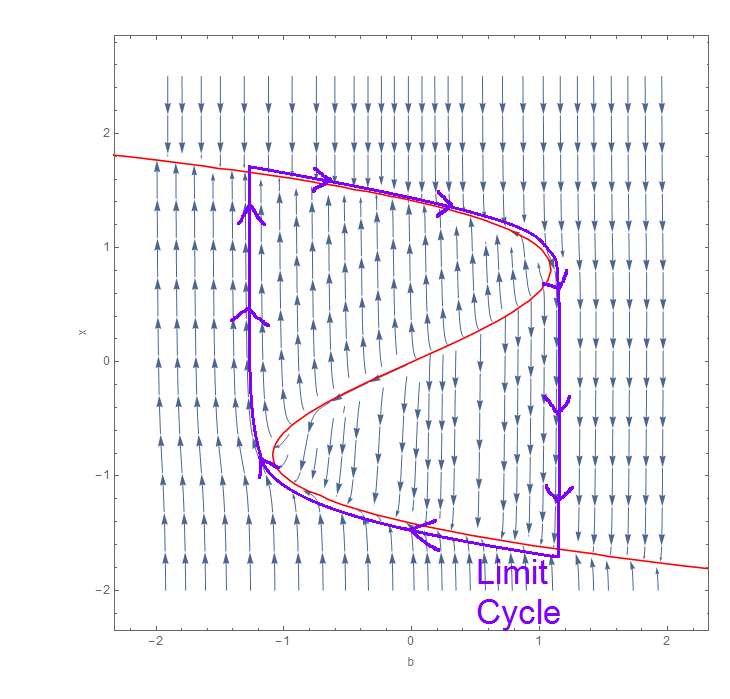 The most important feature of this phase plane is the existence of a single closed trajectory (called a limit cycle) which contains part of the red nullcline. It is not that clear from the first diagram since the trajectories near the red nullcline get cut off, however this limit cycle is highlighted in purple to the left. This is precisely the cycle of a heartbeat! Close to this nullcline, the dynamics are actually quite slow since $\frac{dx}{dt}$ is relatively small, but towards the ‘turning points’ of this nullcline, we see the trajectories become more vertical (due to the threshold and $\epsilon$) and the solution travels much faster.
Well, there we are! Hopefully you’ve all learnt something more about your own hearts. As a bonus for making it to the end, here is a link to one of my favourite songs, Heartbeats by The Knife (I may or may not have written this blog post just to share that).
More from Chalkdust

In conversation with Jonathan Farley
We spoke with Jonathan Farley about his research and experiences as a black mathematician.
Creating hot ice
We created hot ice from scratch, a solution that remains liquid even below its freezing point!
Is it better to run or walk in the rain?
When you're caught in the rain without an umbrella... what is your best option?
Debugging insect dynamics
Explain the strange dynamics of certain insects using game theory
Christmas cracker joke III
Behind today's door... A joke!
The evolutionary arms race
Applying game theory to evolution