
If you’re anything like me, then what I’m about to show you will have you checking the date isn’t April 1st. But no, that mischief-making time is far behind us, and the following is entirely true. Hold onto your logic hats, because we’re going to explore Tupper’s self-referential formula.
Meet the monster
$$\frac12 \lt \left\lfloor \operatorname{mod}\left( \left\lfloor \frac{y}{17}\right\rfloor 2^{-17\left\lfloor x\right\rfloor – \operatorname{mod}(\lfloor y\rfloor,17)}, 2\right)\right\rfloor$$

The Dr. Frankenstein behind this creature is the computer scientist, Jeff Tupper. In a 2001 paper on reliable, two-dimensional computer-graphing algorithms, Tupper introduced this as merely an example; this was just one function that could be plotted with graphing software. To plot this formula, we divide the $(x,y)$ plane into a grid of unit squares, as shown below:
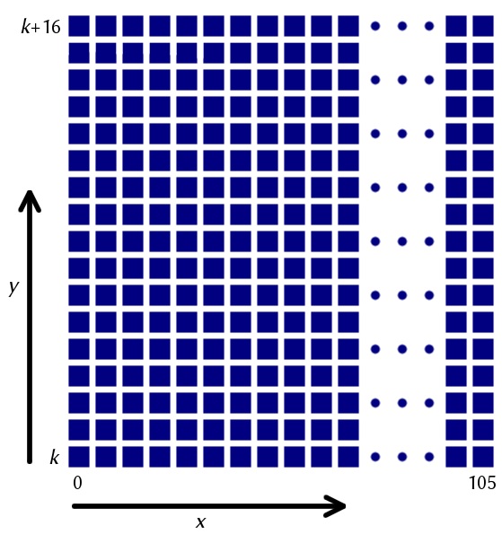 The bottom-left square has value $(0,0)$ and then the one to the right has co-ordinates $(1,0)$, and so on. Essentially, we’re plotting on squares instead of points.
To plot the formula, we need to decide whether we’re going to shade a square or not. Given a square $(x,y)$, we calculate the value of the right-hand side of the inequality and colour the square black if the inequality holds. If the inequality doesn’t hold, we leave the square white. In Tupper’s formula, ‘mod’ refers to modular arithmetic — mod($a,b$) is the remainder when $a$ is divided by $b$. The other funny bit of the formula is the floor function. This is the half square bracket symbol, and returns the largest integer that is less than or equal to the input.
If you plot Tupper’s inequality over squares $0<x<105$, the outcoming is the following:

Image: Wikimedia commons user Larske, CC BY-SA 3.0
I’ll let that sink in for a moment. No, your eyes are not deceiving you — the formula plots a bitmap picture of itself! Hence the name Tupper’s self-referential formula, although Tupper never called it as such in his paper. You’re probably waiting for me to shout ‘April fools!’ but wait, it gets worse!
There is one slight missing detail, however. What is $k$ on the $y$-axis? We seem to be in comfortable terrain on the $x$-axis but in limbo on the $y$-axis. The value of $k$ is the following 543-digit number:
960 939 379 918 958 884 971 672 962 127 852 754 715 004 339 660 129 306 651 505 519 271 702 802 395 266 424 689 642 842 174 350 718 121 267 153 782 770 623 355 993 237 280 874 144 307 891 325 963 941 337 723 487 857 735 749 823 926 629 715 517 173 716 995 165 232 890 538 221 612 403 238 855 866 184 013 235 585 136 048 828 693 337 902 491 454 229 288 667 081 096 184 496 091 705 183 454 067 827 731 551 705 405 381 627 380 967 602 565 625 016 981 482 083 418 783 163 849 115 590 225 610 003 652 351 370 343 874 461 848 378 737 238 198 224 849 863 465 033 159 410 054 974 700 593 138 339 226 497 249 461 751 545 728 366 702 369 745 461 014 655 997 933 798 537 483 143 786 841 806 593 422 227 898 388 722 980 000 748 404 719
I completely lost it at this stage! If you look at the $k$th square on the $y$-axis up to $k+16$th square (providing you ignore everything below and above it), you will see the bitmap image of Tupper’s formula itself. It’s probably time to take an aspirin before you read on.
The plot thickens
In case you found the fact that Tupper’s formula plots an image of itself uninteresting, then let’s take it up a notch. Say we didn’t like our 543-digit $k$ value and wanted to scroll up and down the $y$-axis and see what we get. As you scroll up and down the axis from $-\infty < y < \infty$, Tupper’s formula plots everything.
Yes, everything!
Anything that you can imagine that fits in a 106 × 17 pixel grid is somewhere in the plot of the formula for different $k$-values. Here are some examples:

Just beautiful.
Euler’s identity, found at the equally beautiful value of
k=2352035939949658122140829649197960929306974813625028263292934781954073595495544614140648457342461564887325223455620804204796011434955111022376601635853210476633318991990462192687999109308209472315419713652238185967518731354596984676698288025582563654632501009155760415054499960

The Gaussian integral formula, a beautiful equation but perhaps better displayed in a different font.
The Gaussian integral, with $k$ value
15698740217957008290707879155121161883678974960036820451838496553059304278159396804501767385425557279097842550595147762247567444900095651676508307485805378176431687632652303884950179064554815878189381448932035874145965881631363964883085974756487867902744830960668082577437782189064512907889924899300621786362424181692579651239045992794686365369708864611291854934130524940679843180800552468281283793284632769100458995693741829668924772738264539491965665810196314332016077292880174239602703695648943390464074020112302080

A magazine for the mathematically curious.
A little something for Chalkdust… found at the ‘Chalkdust number’,
4858487703209092733322862398653043018592629026591304793635321373285787870069339390116252383989378150552996946264854676263885000302000180276205526648180456437136216842896260372822447858483709190681349953797852444250304705363038530208929336630045253142258713708305870359636629695250083345580558050487149258713719091145945762431610468728459486026325651076243386252860740825595177362999746722113770762345683083175539003004632104248133147593714665917767442890208302572288879906923054990034030582534708696320319941891397987272291395229158220073271296
From picture to $k$
As previously explained, the plotting of this bitmap function takes place over a series of squares. However, say you had a picture in mind that you wanted to graph and needed to know its corresponding $k$-value. Rather than scrolling randomly until you find it, there is a much more efficient method:
- Beginning in the bottom left hand square of your desired image, allocate a 1 if you want it to be shaded in or a 0 if it should remain blank. Now consider the square directly above and assign either a 1 or 0 in the same way.
- Continue to scroll up the first column. Once the first column is dealt with, move onto the second column beginning with the bottom square again. Repeat the 1,0 allocating.
- Scroll up the second column, then the third, fourth, fifth and so on until you have assigned binary digits to each square in each column of the 106×17 pixel image.
- You will now have an incredibly long binary number (a 1802-digit number to be exact). Convert this number into base 10, and multiply by 17.
- Like magic, you now have your $k$-value.
To try Tupper’s formula for yourself, visit http://damnsoft.org/others/tupper.html and for more information, take a look at Numberphile’s video, The ‘Everything’ Formula.
Chalky comment: the author of this article, Harmeet Singh, published a similar piece last month with Plus Magazine, which is a favourite read of the Chalkdust team!
More from Chalkdust

What’s hot and what’s not, Issue 23
Fashion is fleeting, Chalkdust regulars are not.
Chalkdust dissertation prize winner 2024
Molly Ireland shares her experience of winning our first ever dissertation prize!
In conversation with Martin Hairer
We talk to the Fields medallist about his life, his work and his advice to his younger self.
Chalkdust Book of the Year 2020
We announce the shortlist
Curiosities of linearly ordered sets
Andrei Chekmasov explores order and infinity
John Forbes Nash: the legacy
Exploring the legacy of John Nash (1928 – 2015)