
Believe it or not, I never leave home without my trusty slide rule in my pocket. In the years before 1970, this would have been totally normal for any engineer, with the slide rule being the archetypal symbol of the engineering profession, much like how the stethoscope remains that of the medical profession. However, with the advent of the pocket calculator, the slide rule has completely vanished from public view and its demise is a wonderful example of a paradigm shift, as described by Thomas S Kuhn in The Structure of Scientific Revolutions.
I often get asked “What are you doing with that thing?” when I grab my slide rule to convert miles to kilometres or, once I’ve finished refuelling, to calculate my fuel economy. Most of my students have never seen a slide rule and are at first quite incredulous when I show them my Faber–Castell 62/82N. Not that I’ve ever managed to convince one of them to switch to a slide rule, but at least I normally manage to instil some interest in them for these mathematical instruments.
At the heart of the typical slide rule are logarithms. The first logarithm table was published in 1614 by John Napier of Merchiston (1550–1617) in Mirifici logarithmorum canonis descriptio. Other mathematicians, such as Jost Bürgi, also worked on logarithms and published tables of them in the following years. Logarithms are extremely useful when it comes to the multiplication or division of numbers as they allow you to replace the multiplication of two values, $x$ and $y$, by the sum of their respective logarithms,\begin{equation}
xy=b^{\log_b(x)+\log_b(y)}, \label{e: log}\tag{$*$}
\end{equation}where $b$ represents the base of the logarithm. Today, the most common bases are $b=10$ (the so-called decadic or Briggsian logarithm, named after Henry Briggs, who championed its use); $b=\mathrm{e}$, where $\mathrm{e}$ is Euler’s number (yielding the natural logarithm); and $b=2$ (the logarithmus dualis), which is especially useful in computer science. For our purposes, the base itself is not particularly important and, even if it were, the logarithm to some given base $b$ can easily be determined from that to a different base $b’$ using the formula $$\log_b(x)=\frac{\log_{b’}(x)}{\log_{b’}(b)}.$$
The early days of slide rules
Performing multiplication or division using a logarithm table was, however, still quite time consuming and prone to errors. Firstly, no table was completely error-free as these were calculated and typeset manually. Secondly, looking up values in hundreds of densely typed pages added further complexity. The following picture shows part of a logarithm table from 1889:

As an example, we will try to multiply 6305.7 by 6310 using this table. Firstly, one has to determine the logarithms of these numbers. To do this, these values must be written in the form $mb^E$, where $b$ is the base we are working with, $E$ is the exponent and $m$ is the normalised mantissa, satisfying $1 \leq m < b$. Working in base 10, this yields $6.3057 \times 10^3$ and $6.31 \times 10^3$. If we were to work in binary instead of in the decimal system, this process is exactly the way in which floating point numbers are represented in modern digital computers.
The table is then used to look up the logarithm of the mantissa. For the mantissa corresponding to 6305.7, we go to the entries associated with the 6300 numbers, read down until we reach ’05’ and then across to the column headed ‘7’, which is the decimal part. We find the entry to be ‘7333’, to which we add the prefix ‘799’ (given in the top left hand entry of the table), to obtain the answer $\log_{10}(6.3057) \approx 0.7997333$. In a similar fashion, we get $\log_{10} (6.31) \approx 0.8000294$. So, taking into account that $\log_{10} (10^3) = 3$ and recalling that logarithms turn multiplication into addition, we have\begin{align}\log_{10} (6.3057 \times 10^3) &= \log_{10} (6.3057) + \log_{10} (10^3) \approx 3.7997333,\\
\log_{10} (6.31 \times 10^3) &\approx 3.8000294.\end{align}
Again, referring back to equation (\ref{e: log}): if we are multiplying two numbers, we want to add their logarithms, and so the sum of these values is 7.5997627 and our answer is $10^{7.5997627}$, which we must now convert to something useful. The leading seven is the exponent, so we instantly know that the result must be of the order $10^7$. What we need now is the antilogarithm of 0.5997627, which the logarithm table (not shown here) tells us is approximately 3.9789. So the final result is$$6305.7 \times 6310 \approx 3.9789 \times 10^7 = 39789000,$$which is pretty close to the exact solution 39,788,967.
Slide rules: rise and fall
As you can tell, this technique is pretty laborious and gave rise to various mechanisations that finally led to the slide rule. In 1624, Edmund Gunter (1581–1626) published the brilliant idea of dividing a ruler logarithmically. In the simplest case such a ruler had a scale running from 1 to 10 so that one could work directly with normalised mantissae. To multiply two numbers, their exponents would be determined and added, and then the logarithms of the two normalised mantissae were added by means of dividers, which were used to mark out the lengths on the ruler corresponding to them.
The use of dividers meant that the procedure was still a bit cumbersome. It was greatly simplified by the idea of using two identical rulers, divided logarithmically, which could slide along next to each other. There is still some debate among historians about who actually invented this early slide rule, but most experts give that honour to William Oughtred (1574–1660).
The following picture shows a simple slide rule from the early 20th century with only a few scales. The two bottom scales (quite atypically denoted by E and V), are shown calculating the product $2\times3$.

The scale E is moved across so that it starts at the point 2 on V. The length 3 on E corresponds to the point 6 on V, which is the answer. What we have done is added the length of $\log_{10}(2)$ (on V) to the length $\log_{10}(3)$ (on E) to obtain the correct result. As all operationsvare done with normalised mantissae, a slide rule allows operations with numbers of arbitrary size-one only has to take care of the exponents manually. For multiplication, the exponents are added, while they are subtracted for division. Obviously, to divide two numbers one just has to subtract the lengths of their respective logarithms, so the picture above could also be seen as the calculation $\frac{6}{3}=2$.
One neat feature of a slide rule is that it not only yields a single result but a complete table of results. In the example above we not only got the single answer $6$ but a table showing all multiples of two up to $10$ (the range being restricted by the length of the slide rule). This is extremely handy when one has to convert miles to kilometres-as I often have to do since my car was imported into Germany and still measures distances in miles.
Obviously, a slide rule can’t help with the addition and subtraction of numbers, which has to be done manually, but it can help with much more difficult calculations than just multiplication and division. The following picture shows a more complex slide rule than the one used just. Here, both front and back are filled with scales, hence the name duplex slide rule:
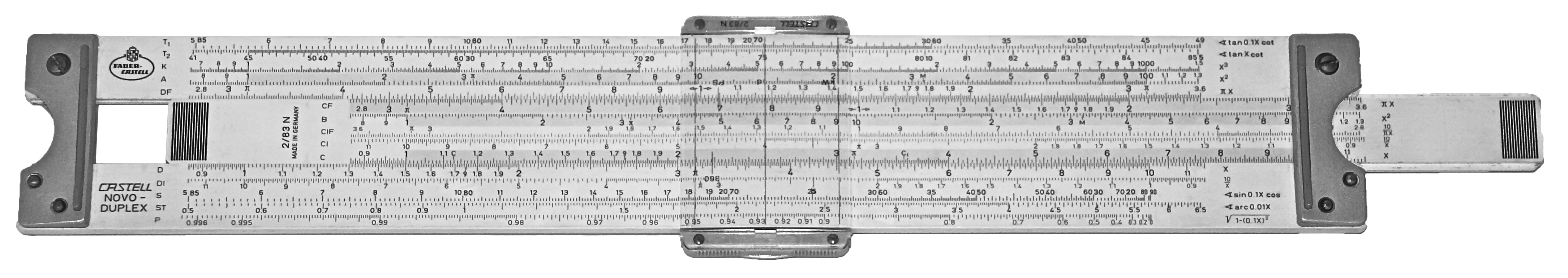
The slide rule below, a Faber–Castell 2/83N, is one of the last and most powerful models ever built. Its front and back feature 30 scales: simple scales for multiplication to more complicated ones like cube scales, several trigonometric scales and double logarithmic scales, which can be used to compute $\sqrt[x]{y}$ and $y^{x}$.

A Faber Castell 2/83N Front
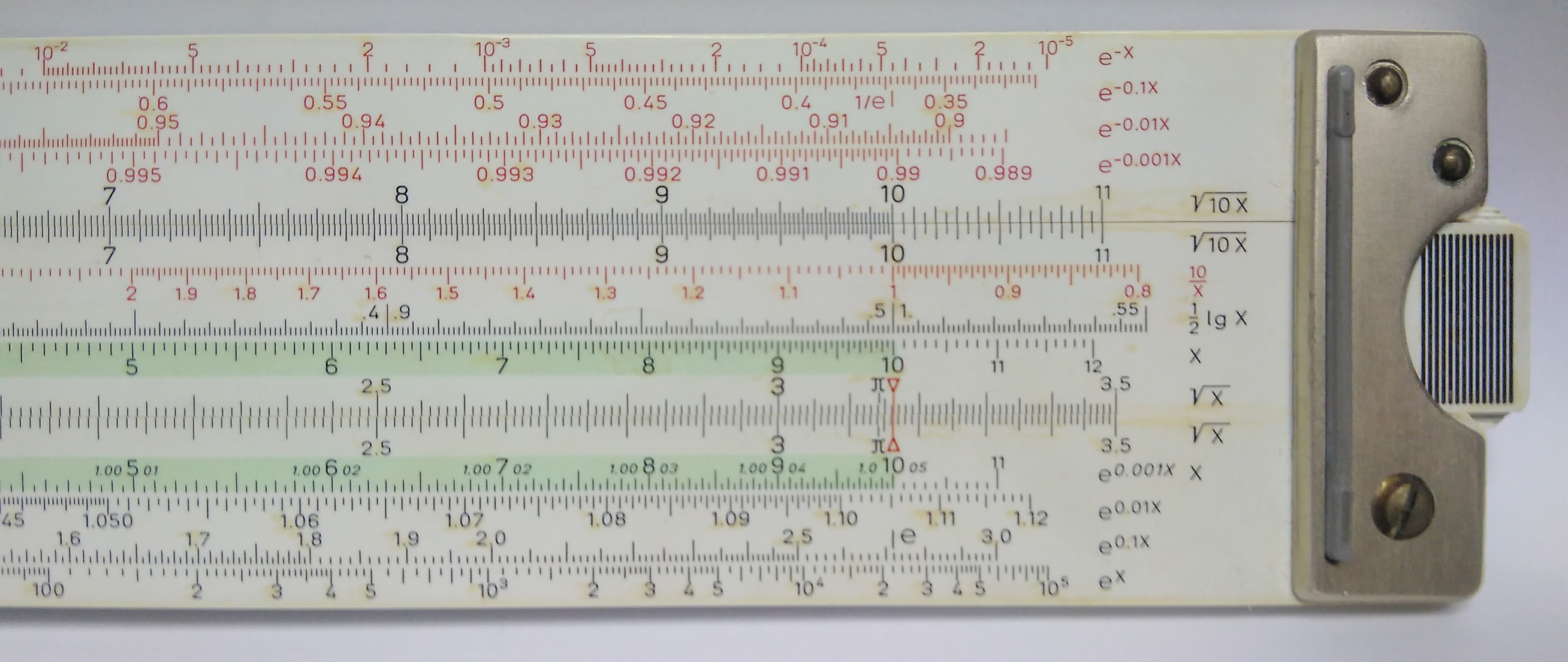
A Faber Castell 2/83N back
Typically, a slide rule also has a movable slider with at least one hairline covering the whole vertical space between the top- and bottommost scale to facilitate readout. This slider often features additional hairlines that are spaced at carefully selected distances to the left and right of the main hairline and allow the instant multiplication of a value by fixed constants. Engineering slide rules, for example, typically have a special-purpose hairline to convert between horsepower and kilowatts. The 2/83N slide rule shown above has many such hairlines, including one allowing you to compute $\log_2(x)$ using the double logarithmic scales: pretty handy in computer science, but a bit ironic given that computer science more or less killed the slide rule.

Flight computer
And, finally, the picture on the right shows one of the rarest and strangest slide rules: a circular slide rule, dating back to the days of the cold war and roughly estimating the number of casualties and catastrophic effects of a nuclear strike.
Nuclear slide rule
So if you ever find a slide rule at a flea market, buy it! You will see that it is a thing of beauty and a joy to use.
More from Chalkdust

In conversation with Bernard Silverman
We chat to the chief scientific advisor to the Home Office about the role of scientists and mathematicians in politics
Linear algebra… with diagrams
Rediscover linear algebra by playing with circuit diagrams
Debugging insect dynamics
Explain the strange dynamics of certain insects using game theory
Variations on Fermat: an agony in four fits
Fermat's Last Theorem with complex powers, wrapped in a story every mathematician can relate to
The simplest difficult task
Factorisation is often used in cryptography. But there's something even simpler which turns out to be just as hard.
Origami tesseract
Folding origami, building networks, making projections and multiple dimensions!