
- This article has code for you to run! Skip to the downloads.
Imagine that we have a group of 20 volunteers. We give all 20 people identical pills, and measure a response in each of the people. The responses would not all be the same—there is always some variability. If we divide the 20 responses randomly into two groups of 10, the means of the two groups will therefore not be identical.
If we had instead given each group of 10 people different pills (say drug A and drug B) then we would also find that the means of the two groups differed. If drug A was better than B then the mean response of the 10 people given A would be bigger than the mean of the 10 responses to B. But of course the response of group A might well have been bigger, even if drugs A and B were actually identical pills.
It is one of the jobs of applied statisticians to tell us how to distinguish between random variability and real effects. They can tell us how big the difference between the means for A and B must be before we believe that A is really better than B and not just the result of random variability.
It is the aim of this article to persuade you that the ways of doing this that are commonly taught give rise to far more wrong decisions than most people realise. This is not trivial. It gives rise to the publication of discoveries that are untrue. For example, it may result in the approval of medical treatments that don’t work.
How to tell whether an effect is real, or mere chance
In the example above, the 10 people who were given drug A were chosen at random from the 20 volunteers. If the two drugs were in fact identical then each of the 20 people would have given the same response regardless of whether they had been allocated to the A group or the B group. The response would be a characteristic of the person, and not dependent on whether they got pill A or pill B. So the observed difference between means would depend only on which particular individuals were allocated to group A or B, i.e. on how the random numbers came up. Therefore it makes sense to look at the outcomes that would have been observed if the random numbers had been different.
There are 184,756 ways of selecting 10 observations from 20, giving 184,756 differences between means that are what we would expect to observe if in fact the treatments were identical. The speed of computers is such that they can all be inspected in just a few seconds. Figure 1 shows the distribution of all 184,756 differences between means. Since it is based on the premise that the treatments were identical, the average difference between means is zero.
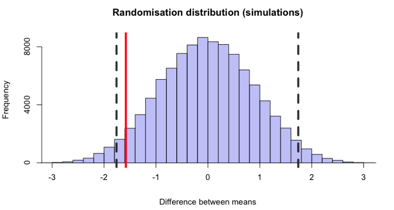
Figure 1: A randomisation distribution. It shows the distribution of all 184,756 differences between means for every possible way of choosing 10 observations from 20, based on the assumption that the pills are identical, so the mean of the distribution is zero. The vertical dashed lines mark 2.5% of the area in the lower tail and 2.5% in the upper tail. The red line marks the difference between means that was observed in the experiment. Because the red line lies between the dashed lines we can conclude that there is not strong evidence to say that the true difference is not zero.
The observed mean response to the 10 people on drug A was 0.75, and the mean for drug B was 2.33. So the observed difference between means was 0.75 – 2.33 = –1.58. This value is marked by the vertical red line in Figure 1. About 4% of the differences are below the observed value, –1.58. Another 4% are above +1.58. So we find that if the two drugs were identical there would be a probability of $p = 0.08$ of finding a difference between means, in either direction, as big as that observed, or even bigger. This 8% is termed the p-value. If it is small enough we reject the premise that the two treatments are identical. And 8% is not really very small: the experiment doesn’t provide strong evidence against the idea that the drugs are identical. This procedure is known as a randomisation test.

William Sealy Gossett (‘Student’)
This sort of problem would be more commonly analysed using a Student’s t-test. This test was invented at UCL in 1908, by William Sealy Gossett, who wrote under the pseudonym ‘Student’. He was chief brewer at Guinness. On a visit to UCL, to work with Karl Pearson, he derived the first test of significance that was valid for small samples and the data used in Figure 1 is from a paper by Cushny & Peebles (1905) and was later used in the paper that first described the t-test (Student, 1908). (Cushny was the first professor of pharmacology at UCL.) It was pioneering work, but it should now be replaced by the randomisation test described here, which makes fewer assumptions. In this case, the samples are sufficiently large that the result of the t-test ($p = 0.079$) is essentially the same as what we obtained.
The postulate that the treatments are identical is called the null hypothesis, and this approach to inference—attempting to falsify the null hypothesis—has been the standard for over a century. It’s perfectly logical.
What could possibly go wrong?
The problems of null hypothesis testing
The $p$-value does exactly what it claims. If it is very small, then it’s unlikely that the null hypothesis is true. Falsifying hypotheses is how science works. Every scientist should be doing their best to falsify their pet hypothesis (the fact that many don’t is one of the problems of science, but that’s not what we are talking about here).
The real problem lies in the fact that the p-value doesn’t answer the question that most experimenters want to ask.
So how small must the p-value be before you can reject the null hypothesis with confidence? A convention has grown that $p = 0.05$ is some sort of magic cut off value. If an experiment gives $p < 0.05$ the result is declared to be “significant” with the implication that the effect is real. If $p > 0.05$ the result is labelled “not significant”. This practice is almost universal among biologists, despite being obvious nonsense—clearly the interpretation of $p = 0.04$ should be much the same as $p = 0.06$.
But that is only the beginning of the problems. The real problem lies in the fact that the p-value doesn’t answer the question that most experimenters want to ask. What I want to know is ‘if I claim, on the basis of my experimental results to have made a discovery, how likely is it that I’m wrong?”. If you claim to have made a discovery (like drug B works better than drug A), but all you are seeing is random variability, then you make a fool of yourself. And the aim of statistics is to prevent you from making a fool of yourself too often.
If you ask most people what the p-value means, you’ll very often get an answer like ‘it’s the probability that you are wrong’.
It isn’t, and I’ll explain why.
The crucial point is that the p-value only tells you about what you’d expect if the null hypothesis were true. It says nothing about what would happen if it wasn’t true. Paraphrasing the words of Sellke et al. (2001),
‘Knowing that the data are “rare” when there is no true difference is of little use unless one determines whether or not they are also “rare” when there is a true difference.’
Let’s define the probability that we are wrong if we claim an effect is real as the false discovery rate (or the false positive rate). That is what we want to know, but it is quite different from the p-value, and it is less straightforward to calculate. In fact it is impossible to give an exact value for the false discovery rate for any particular experiment. But we can make the following statement:
If we declare that we have made a discovery when we observe $p = 0.047$, then we have at least a (roughly) 30% chance of being wrong.
In other words, when we use $p = 0.05$ as a criterion for declaring that we have discovered something, we’ll be wrong far more often than 5% of the time. That alone must make a large contribution to the much-publicised lack of reproducibility in some branches of science. The paper by Stanford epidemiologist, John Ioannidis, Why most published research findings are false touched a nerve. It has been cited over 3,000 times. Of course, he wasn’t talking about all science; just about some parts of biomedical research.
Why p-values exaggerate the strength of evidence
Take the simplest possible example. Let’s ask what the false discovery rate is if we do a single test and obtain the result $p = 0.047$. Many people would declare the result to be (statistically) significant, and claim that the effect they were seeing was unlikely to be a result of chance.
We can treat the problem of significance testing as being analogous to screening tests, which are intended to detect whether or not you have some illness. In screening we need to know about false positive tests—the fraction of all tests that say you are ill when you are not—because it is distressing and expensive to be told you are ill when you’re not.
If only 1% of the population suffer from the disease then a staggering 86% of positive tests are wrong!
There are three things that need to be specified in order to work out the false positive rate for a screening test: these are the specificity of the test, the sensitivity of the test, and the prevalence of the condition you are trying to detect in the whole population that you’re testing. The specificity of a test is the percentage of negative results identified correctly. For example, a screening test with a specificity of 95% means that 95% of people who haven’t got the disease test, correctly, negative. The remaining 5% are false positives: the test says that they have the disease whereas in reality they don’t. That sounds quite good. The sensitivity of the test is the percentage of positive results identified correctly: you have a disease and the test agrees. So, if the sensitivity is 80%, then if you have the disease, you have an 80% chance that it will be detected correctly. That also doesn’t sound too bad.
However, if the condition that you are trying to detect is rare (the prevalence of that condition), then most positive tests will be false positives. For example, the screening test for mild cognitive impairment (which may or may not lead to Alzheimer’s disease) has the specificity and sensitivity given above, but if only 1% of the population suffer from the disease then a staggering 86% of positive tests are wrong! This happens because most people haven’t got the disease and so the 5% of false positives from them overwhelms the small number of true positives from the small number of people who actually
have the disease. This is why screening for rare conditions rarely works.
Now we can get to the point. How does all this apply to tests of significance? Figure 2 shows an argument that’s directly analogous to that used for screening tests.

Again we need three things to get the answer. The first two are easy. The probability of getting a false positive when there is no effect is simply the significance level, which we have seen is normally set to 0.05. It’s the same thing as (1 – specificity) in the screening test example. The power of the test is the probability that we’ll detect an effect when it’sreally there. It’s the same thing as the sensitivity of a screening test. It depends on the variability and the size of the effect. The sample size is customarily chosen to give a power of 0.8 (as in Figure 2) though it’s very common for sample sizes to be too small, so the power of many published tests is actually in the range 0.2–0.5.
The third thing that we need is the tricky one. In order to work out the false discovery rate, we need an analogue of the prevalence in the screening test example. In the case of screening, that was simply the proportion of the population that suffered from the condition. In the case of significance tests, the prevalence is the proportion of tests in which there is a real effect, i.e. the null hypothesis is false. If one were testing a series of drugs, you’d be very lucky if the proportion that worked was as high as 10\%; so, for the sake of an example, let’s take the prevalence to be 0.1.
 We can now work though the example in Figure 2. If you do 1,000 tests, then our prevalence means that in 900 (90%) of them the null hypothesis is true (there is no effect) and in 100 of them (10%) there is a real effect. Of the 900 tests in which there is no real effect, applying the significance level of 5% means that 45 of them will give $p < 0.05$: they are false positives and we’d have claimed to have found a result that isn’t there. That is as far as you can get with classical null hypothesis testing. But to work out what fraction of positive tests are false positives we need to think about not only what happens when the null hypothesis is true (the lower arm in Figure 2), but also what happens when it is false (the upper arm in Figure 2). The upper arm has 100 cases where there is a real effect and, due to the power (or sensitivity of the test), 80% of these are detected (i.e. give $p < 0.05$), so there are 80 true positive tests.
Therefore the total number of positive tests is 45 + 80 = 125, of which 45 are false positives. So the probability that a positive test is actually false is $45/125 = 36\%$. This is far bigger than the 5% significance level might suggest.
If you claim a discovery on the basis that $p = 0.047$ you’ll be wrong at least 26% of the time… and maybe much more often.
The argument in Figure 2 shows that there is a problem, but it still doesn’t quite answer the original question: what’s the false discovery rate if we do a single test and obtain the result $p = 0.047$? To answer that, we need to look only at those tests that give $p = 0.047$ (rather than all tests that give $p < 0.05$, as in Figure 2). This is easy to do by simulation (see the R script on our website). The result is that if you claim a discovery on the basis that $p = 0.047$ you’ll be wrong at least 26% of the time (that’s for a prevalence of 0.5), and maybe much more often. For a prevalence of 0.1 (as in Figure 2) a staggering 76% of such tests will be false positives.
What is the prevalence of true effects?
The biggest problem with trying to estimate the false discovery rate is that the prevalence of true effects is unknown. It is what a Bayesian would call the prior probability that there is a real effect (‘prior’ meaning the probability before the experiment has been done). As soon as the word Bayes is mentioned, statisticians tend to relapse into arguing amongst themselves about the principles of inference: this is unhelpful to experimenters. In my opinion, it is not acceptable (in the absence of strong empirical evidence) to assume that your hypothesis has a chance of being true that’s more than 50% before the experiment has been done. If you did then it would be tantamount to claiming that you had made a discovery and justifying that claim by using a statistical argument that assumed that you were likely to be right before you even did the experiment! Most editors and readers would reject such an argument, but they are happy to accept marginal p-values as evidence.
This alone may explain why so much research has proved to be wrong.
Resources and downloads
- Original paper
- Two pieces of R code written by David which you can use to run your own simulations to convince yourself of the risks of using the p-value when reporting results:
- Instructions
- 2-sample-rantest-exact.R
Uses random sampling with replacement to generate the randomisation. This was used to generate Figure 1. - two_sample_randtest.R
Lists all possible allocations of a sample of 10 from 20 observations. The number of combinations is given by ncom = $\binom{20}{10}$ = 187,456.
It takes a very short time to look at all of them. The results are essentially the same with both programs.
YouTube presentation
- David explains the perils of p-values in this online presentation:
References and further reading
- Colquhoun D (1971). Lectures on Biostatistics Clarendon Press, Oxford
- Colquhoun D (2014). An investigation of the false discovery rate and the misinterpretation of p-values. R Soc Open Sci 1, 140216
- Cushny AR & Peebles AR (1905). The action of optical isomers: II. Hyoscines. J Physiol 32, 501–510
- Ioannidis J (2005). Why most published research findings are false. PLoS Med 2, 696–701
- Sellke et al. (2001). Calibration of p-values for testing precise null hypotheses. The American Statistician 55, 52–71
- Senn S & Richardson W (1994). The first t-test. Stat Med 13, 785–803 (£)
- Student (1908). On the probable error of a mean. Biometrika 6, 1–25
More from Chalkdust

John Forbes Nash: the legacy
Exploring the legacy of John Nash (1928 – 2015)
Fermat Point by Suman Vaze
The maths behind Issue 02's cover
In conversation with Artur Avila
Chatting with a Fields Medallist in a Leicester Square pub
The joys of the Jacobian
Robert Smith? tells us how his favourite matrix saves lives
The Mpemba paradox
Why does warm water freeze faster than cold water?
Breaking out of the prisoner’s dilemma
What happens if you play the prisoners' dilemma against yourself?