Reproduce or die - Chalkdust

1 August 2019

It was about 1975 when I first heard of John Conway’s Game of life, a cellular automaton that is able to mimic aspects of living organisms, such as moving, reproducing and dying. Some school friends who had joined the computer club awoke my curiosity and even though I didn’t know the exact rules at the time, I made up my own version and called it: Reproduce or die 2/4. Let me explain.

John Conway’s version takes place in an infinite 2D checkerboard universe where time goes by in discrete steps. Each square or ‘cell’ in his universe has two possible states, either alive or dead. An initial configuration of living cells is created and the state of any cell at the next time step depends on how many living neighbouring cells it has at the current moment. Conway included all eight neighbouring cells surrounding the one being considered (see the green cell in the figure below), called the Moore neighbourhood. There are four cells touching its sides (labelled s in the figure): north, south, east and west and four neighbouring cells touching corners (labelled c) with the cell in question: NE, NW, SE and SW. If a cell has just two living neighbours, it will stay alive or stay dead. If it has three living neighbours, it will stay alive or come alive. Any other total and it will die or stay dead. For more about Conway’s version, check out this link.

Neighbouring cells.

In my checkerboard 2D universe, I only consider the 4 side cells that surround a living cell, i.e. the ones north, south, east and west (the cells marked ‘s’ above), known as the Von Neumann neighbourhood. I ignore the corner cells (marked ‘c’). The rules are simple:

If a living cell has exactly two living side neighbours in the present time step (or generation as I call it), then two new daughter cells are born into the two empty side cells (i.e. they come alive) and the parent stays alive in the next generation.
Every other cell dies or stays dead in the next generation.

As the only cells that survive are ones that have two out of four possible living neighbours and they also reproduce (all others dying), I call my version Reproduce or Die 2/4. At first I worked out the new generations by hand on graph paper, but when home computers became a reality in the early 1980’s, I wrote my own programs.

Applying the rules

Consider three living cells in a row (below left, shown in green) in the first generation. The end ones have only one neighbour each so they will die. The middle cell has two neighbours so will live and at the same time will produce two offspring, one in each of the empty neighbours cells (marked ‘0’), one above and one below (see middle figure below). A new shape is created, which is also a line of three living cells but this time vertical. In the next generation, only the middle cell will survive and will create two daughter cells, one to the left and one to the right. The ‘organism’ returns to its original shape (below right) and then repeats the cycle continuously. It is an oscillator of period 2. I call it the rod.

The evolution of the ‘rod’, from left to right.

Consider now a set of three living cells that make a small corner (below left). The end cells each have only one neighbour (the corner cell itself) so will die, but the middle cell that makes the corner has two neighbours so will live and give birth to two daughter cells, one in each of the two unoccupied side cells. The new shape is still a corner, but pointing the other way. In the next generation, the end cells will die and the middle cell will reproduce offspring into the two empty side cells and voila, we get the same starting shape again. This too is an oscillator of period two. I call this shape the corner. Every birth that is possible in this universe is built up of just these two: the rod and the corner.

The evolution of the ‘corner’, from left to right.

For simplicity, the chosen universe for the remainder of this article has a finite size (20×20 cells) but has periodic boundary conditions, like some video games. This means that the top of the spreadsheet is connected to the bottom and the right side is connected to the left side, so the universe is like the surface of a torus. Let us now see what kind of creatures can inhabit this cosmic doughnut when we start combining more than three living cells next to each other.

Shakers and movers

Five oscillators of period two. Clockwise from top: corner, rod, H, and the small and large butterflies. The grid on the right shows the second generation of each oscillator.

The Reproduce or die 2/4 universe cannot be static, due to the chosen rules and in its simplest state it has to at least oscillate, so let us have a look at a few of the ‘shakers’ that live here. Five oscillators are shown above.

The ‘corner’ and ‘rod’ have already been introduced. Each has a period of two and both are among the most common shapes to turn up in random initial conditions i.e. those where the initial state of each cell is chosen at random. The H also has a period of two. The ‘large and small butterflies’ shown above also have periods of two and seem quite rare, but have appeared as end products of a symmetric explosion (see later).

A good game of life would be boring if it didn’t have any mobile creatures, so fortunately this universe has a fair share of travelling folk. Four examples are shown below. In this case all move north:

Gliders that move north. Four time-steps are shown, going clockwise from top left. The gliders are called (clockwise from bottom left in the first time-step) the small C, the hat, the short leg, and the leg1.2.3.2.

The first glider (bottom left) I call the small C. It evolves over three generations before returning to its original shape, but it has moved one cell north during this period. It thus has a speed 1/3 that of light and a period of 3. (Note: speed of light is the name given to the maximum possible speed, which in this universe is one cell per time interval). The small C is very different to all the other gliders so far discovered, as will become clear. The next glider (above the C), I call the hat. It keeps the same shape every generation (so has a period of one) and moves at the speed of light: one cell per time step. It is the most common glider in this version of the Game of Life. The top right shape in, I call the short leg, which is like the hat but with one short limb. It has a period of two and moves at the speed of light. The final example (bottom right shape) is the leg1.2.3.2. This one has a period of 4 before it returns to its initial shape and like almost every glider it moves at the speed of light.

As with John Conway’s Game of Life, this version also has shapes that create strings of gliders (guns as they are called), plus there are many interesting collisions involving moving shapes, but time and space are limited so let us move onto one of the more spectacular performances in the presentation.

The big bang

There is a category of simple regular shapes that grow like an explosion and maintain their symmetry through each ensuing generation. I call the simplest one, starting with a 2×2 array of living cells, the ‘big bang’. A selection of stages of this explosion is shown below. Each generation might make a unique repeating floor tile, or possibly, one of the most challenging crosswords layouts ever!

The big bang on the 1st, 11th, 21st, 41st, 81st and 136th generation.

In an infinite universe, all such shapes would grow indefinitely, but as it is finite here, the advancing ‘shock waves’ of the exploding shapes meet each other at the edges and then interfere. The big bang eventually settles down to a simple oscillating pattern of 12 corners on the 136th generation, much like the formation of the galaxies (or stars) in our own universe. All other symmetrical patterns settle down, but some with a long dance, needing up to seven generations in the end repeating cycle.

A random field

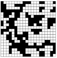
A random initial field.

A random field is one where the initial state of the cells, alive or dead is decided by a probability rating $p$, e.g. $p = 0.5$ would mean the chance of a cell starting alive would be 50%, hence about 50% of the cells would be alive using a random number function at the start. Most random, asymmetric shapes produce what seem to be permanent disorder that expands and fills the space and looks like it never wants to settle down. As this particular universe is finite in size, then there are a finite number of possible states, so in fact all configurations will repeat, even if they take a long time. To the right is a typical example of such a random population many generations after its creation. In this example one can see, top right, an oscillating corner, while near the centre is a hat glider, moving downwards. Neither shape will survive more than a generation or two, but this is how precarious life is in this universe.

Conclusion

The Reproduce or die 2/4 variation does have its moments of oscillators, gliders, guns, collisions and explosions, with some amazing kaleidoscopic patterns to delight the eyes. The downside is that there are far too many uncontrolled population growths that swamp and destroy the more interesting order. Life in such volatile fields is short-lived and fleeting, much like the real universe. Perhaps that is what makes this kind of life so precious.

Whatever next?!

In Reproduce or die 2/4, there are a few questions I would like to ask:

How would changing the finite size of the universe change the outcomes? I used a 20×20 universe, but I’d expect it to be different for, say a 30×30. Readers will have a chance to try this out!
In a random field, is there a pattern to the population density?
What is the frequency of appearance of stable shapes, like the hat, corner and rod?
What would happen if the Reproduce or die 2/4 rules were modified slightly? For example when two cells are trying to be born into the same square, what if they cancelled out and it remained empty? That might dampen down those unwanted exponential explosions.

I asked one of my physics students, Dmitry Mikhailov, to create the Reproduce or Die world so readers could play with it themselves. He kindly took up the challenge and has made an interactive version here. All images in this article are also thanks to his program and Dmitry’s contribution is much appreciated.

Please share your discoveries of any interesting news shapes. Remember, stable shapes are hard to find as most situations end in disarray, so don’t be put off (unless you like entropy!). Finally, why not consider trying to create your own set of rules and you can then be the god (or goddess) of your own universe!

Hugh Duncan

Hugh Duncan graduated from UCL having studied astronomy. He taught physics and maths at the International School of Nice for over thirty years. Hugh was a punk when he started UCL in 1976 and guess what, he still is! Check out his band Old Age Spies on YouTube. He recently retired and has just had his first science fantasy book published ‘Life On Mars – The Vikings Are Coming’ inspired by his time at UCL. Check it out too!